Figures & data
Figure 1. Feature-free process planning for milling (Nelaturi et al., Citation2015). At every fixturing orientation, the maximal removable volume (MRV) is computed. Different plans (two of them shown here) remove the same MRVs in different fixturing orders. The top plans with the minimum cost are found.
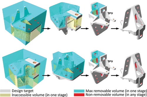
Figure 2. There are 4 main components in our end-to-end process planner for turning: 1) identifying turning axes; 2) fixturing considerations; 3) turning action generation; and 4) turning process planning; discussed in Sections 3.1, 3.2, 3.3, and 3.4, respectively. The 3D models in this and following figures are imaginary parts created in Onshape (https://www.onshape.com/).
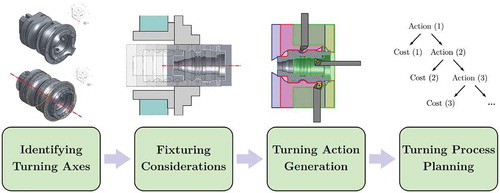
Figure 3. Converting a given target part in (a) to its TC in (b), by sweeping the part for a full rotation around a given axis a (dash-dot red line). The resulting superset (i.e, larger part) can be potentially manufactured by pure turning with the right combinations of tools, and leaves as little volume as possible for other pre-/post-processing machining operations. The same part is shown from two views (top and bottom).
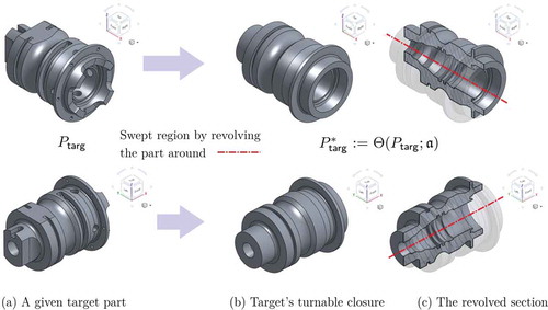
Figure 4. An investigation of the CAD model leads to a set of candidate axes, e.g., of cylindrical faces in this example. One clearly stands out as it results in the smallest TC.
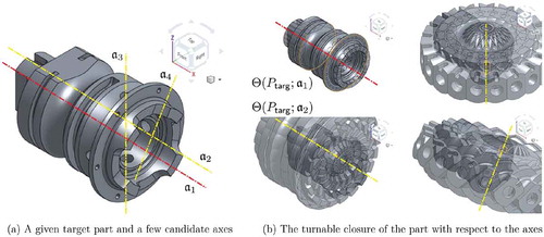
Figure 5. The explicit approach to determining the TC requires projecting a large number of longitudinal sections onto the same 2D plan and computing their union.

Figure 6. The implicit approach to determining the TC requires a PMC test against it, which is obtained by performing intersection tests between orbits and the solid.
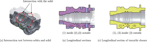
Figure 7. The first transformation positions and orients the part’s TC to align with the machine axis in (a). The different grip configurations are obtained by a discrete set of subsequent rigid transformations (b–d) which are screw motions (top) with or without an additional flip of axis direction (bottom).
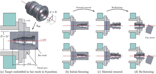
Figure 8. A simplified sketch of the stationary, rotating, and sliding components in the workspace of a simple lathe machine. The planar motion of the sliding components is measure from their 0-position, arbitrarily chosen to be at the world coordinate system’s origin (i.e., spindle center).
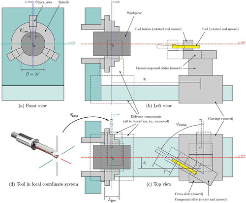
Figure 9. The MTVs for different tool profiles and setup configurations with the same grip/fixturing configuration. The computations are reduced to Minkowski operations on the longitudinal sections.
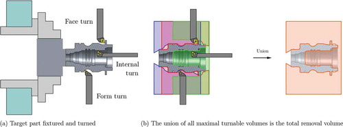
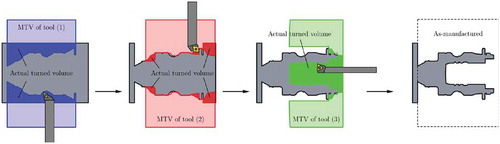
Figure 10. An example turning process plan. The intersection of the MTV with the workpiece at each intermediate state is the actual turned volume, which is used to estimate the cost of that step.