The effect of groove and notch tip angles on testing fracture toughness by SEVNB method: models and experimental validation

Figures & data

Figure 1. SEM image of the groove and V-notch tilted by 30° [12]. Two angles, θ₁, and θ₂, were used to control the morphology of the groove and V-notch, respectively.

Figure 2. Schematic diagrams of the three models; (a) ideal crack model, (b) non-crack model, (c) groove model. u is the groove length, l is the crack length, V_n is the V-notch length, a is the overall length of the flaw, defined as a = u + l + V_n. In the ideal crack model (a), u = 0, V_n = 0, and a = l; In the non-crack model (b), l = 0, a = u + V_n; In the groove model (c), V_n = 0, a = u + l.

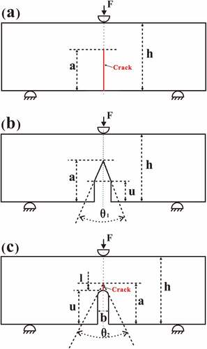
Figure 3. Grid-independent test of ideal crack model, (a) model diagram and node setting method and (b) global mesh generation map and enlarged mesh distribution map of the crack tip.

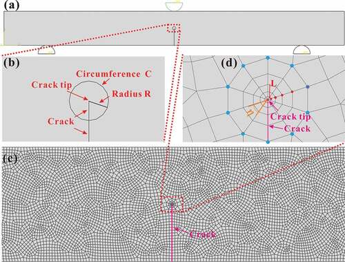
Figure 4. Variation of J-integral for an ideal crack model with varying angle (η).

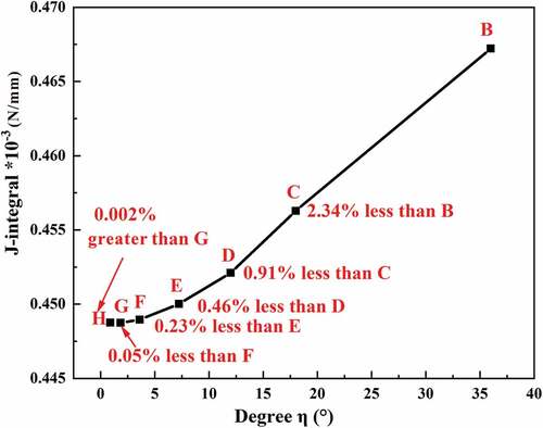
Figure 5. Global stress cloud image of ideal crack model and its stress cloud image enlarged at the crack tip.

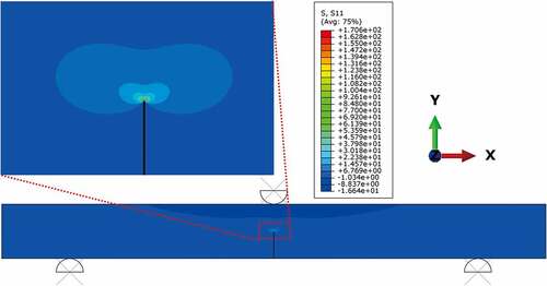
Table 1. Grid-independent test of ideal crack model.

Item	Number of nodes on circumference C	Number of nodes on radius R	Length of L (μm)	Degree η (°)	Global element size (mm)	Number of global elements	Value of J-integral ×10^−3
A	10	5	15.296	36	0.10	19,906	0.4671870
B	10	5	15.296	36	0.05	78,173	0.4672230
C	20	10	4.894	18	0.05	78,707	0.4562888
D	30	20	2.504	12	0.05	80,313	0.4521192
E	50	30	1.628	7.231	0.05	83,747	0.4500180
F	100	50	1.603	3.616	0.05	92,223	0.4489621
G	200	80	1.003	1.852	0.05	112,833	0.4487524
H	400	200	0.402	0.816–1.088	0.05	198,819	0.4487597
I	100	50	1.603	3.616	0.04	136,051	0.4488960
J	100	50	1.603	3.616	0.03	242,055	0.4488455

Table 2. Reference values of model material parameters [23].

Mechanical property	parameters
Young’s modulus, E (GPa)	210
Poisson’s ratio, ν	0.31
Density (g/cm^3)	6.05

Figure 6. Comparison of LFEM results with Equation (2)(2) $K_{IC}=Y\left[\frac{F\times s}{B\times h^{\frac{3}{2}}}\right]\left[\frac{3\times {\left(\frac{a}{h}\right)}^{\frac{1}{2}}}{2\times {\left(1-\frac{a}{h}\right)}^{\frac{3}{2}}}\right]$(2) based on the ideal crack model for three-point bending configuration.

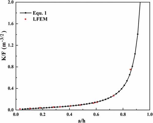
Figure 7. Typical tensile stress distribution of (a) ideal crack model and (b) non-crack model with a V-notch tip angle θ₁ of 90°in a two-dimensional three -point bending beam by LFEM.

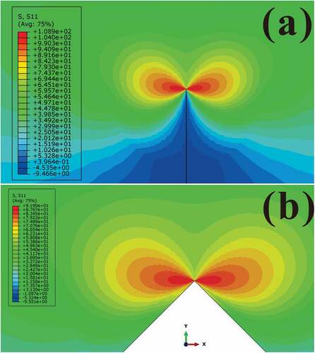
Figure 8. J-integral values of non-crack model with different u/a values and the stress cloud near the V-notch tip with (a) u/a = 0, (b) 0.5 and (c) 0.95, where the angle of the V-notch tip was maintained at 60°. The results when the angle of the V-notch tip θ₁ was 30°, 90°, and 120° were the same as those at 60°, and they are not shown here.

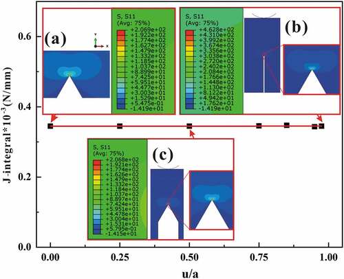
Figure 9. K_Ic/θ1/K_Ic/th for various angles θ₁ (a) and (b) fitted curve. Very good agreement was achieved with the data obtained from the non-crack model.

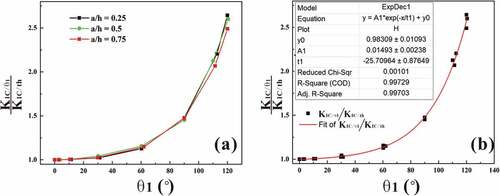
Figure 10. (a) Stress cloud image of a typical ideal crack tip including two marked angles. The stress in the area for a 30° angle was close to zero, while the 60° angle included a large local stress area. Stress cloud image of non-crack models with θ₁ value of (b) 10°, (c) 30°, (d) 60°, (e) 90°, and (f) 120°.

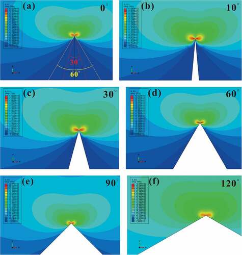
Figure 11. K_Ic/θ2/K_Ic/th for various values of angle θ₂ (a) and the (d) fitted curve. Excellent agreement with the data was obtained by the groove model.

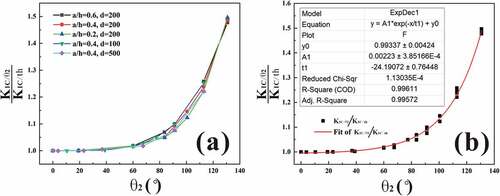
Figure 12. (a) Stress cloud images of a typical ideal crack tip. Stress cloud image of groove models with θ₂ of (b) 19°, (c) 60°, (d) 91°, (e) 113°, and (f) 131°.

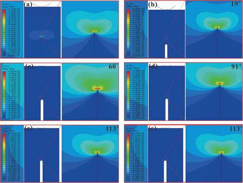
Figure 13. SEM images of the samples of (a) 2.3Y-TZP, (b) 3Y-TZP and (c) Al₂O_3.

Figure 14. Experimental curve and curve predicted by Equationn (6)(6) $\frac{K_{Ic/\theta 2}}{K_{Ic/th}}=0.00223\times EXP\left(\frac{{\theta }_2}{24.19072}\right)+0.99337$(6) of the fracture toughness: (a) 2.3Y-TZP, (b) 3Y-TZP, and (c) Al₂O_3.

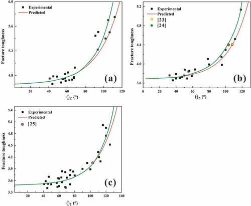
Figure 15. The XRD patterns of the (a) 2.3Y-TZP and(b) 3Y-TZP for the polished surface and fractured surface after fracture toughness testing. V_{m, polished surface} denotes the volume fraction of the phase transformation on the polished surface of the sample. V_{m, fractured surface 1} is the volume fraction of the phase transformation on the fractured surface of the samples with small θ₂, while V_{m, fractured surface 2} is the volume fraction of the phase transformation on the fractured surface of the sample with a large θ₂. m: monoclinic phase of zirconia, t: tetragonal phase of zirconia.

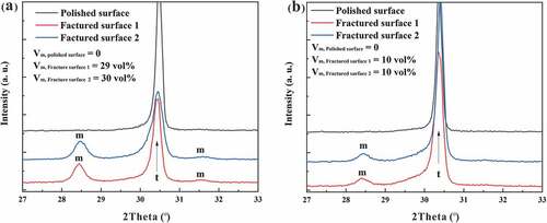
Figure 16. SEM images of (a) 3Y-TZP [27], (b) Al₂O₃ [29], and (c) 3Y-TZP [28] samples with grooves and V-notches.

Table 3. Fracture toughness of 2.3Y-TZP, 3Y-TZP and Al₂O₃ samples.

Sample	Experimental fracture toughness values with θ2 less than 50°MPa•m^1/2		Fracture toughness predicted by Equation (6)(6) $\frac{K_{Ic/\theta 2}}{K_{Ic/th}}=0.00223\times EXP\left(\frac{{\theta }_2}{24.19072}\right)+0.99337$(6) MPa•m^1/2	Fracture toughness predicted by Equation (5)(5) $\frac{K_{Ic/\theta 1}}{K_{Ic/th}}=0.01493\times EXP\left(\frac{{\theta }_1}{25.70964}\right)+0.98309$(5) and Equation (6) /MPa•m^1/2
	Average	Range
2.3Y-TZP	4.74 ± 0.06	4.66–4.82	4.68	4.54–4.61
3Y-TZP	3.76 ± 0.07	3.66–3.88	3.71	3.60–3.65
Al2O3	3.54 ± 0.09	3.41–3.70	3.50	3.40–3.45

Figure 17. (a) Experimental and predicted curves of K_Ic in ZrB₂ and ZrB₂-SiC specimens with various θ₁ and θ₂ values [17]. Images of the notched test bars with θ₁ of (b) 3°, (c) θ₁ of 20°, (d) θ₁ and θ₂ of 9° and 50°, respectively, and (e) θ₁ and θ₂ of 21° and 140° [17], respectively.

Table 4. Fracture toughness values of materials with different θ₁ and θ₂ values.

Sample	Model type for SEVNB Method	θ1	θ2	Test method for$K_{IC/SEVNB}$	Test method for ${\mathrm{K}}_{IC/Ref}$	Fracture toughness rate		Ref.
						$\frac{K_{IC/SEVNB}}{{\mathrm{K}}_{IC/Ref}}$	$\frac{K_{IC/SEVNB}}{{\mathrm{K}}_{IC/th}}$
Tungsten alloy	1	3		SEVNB	SENB-S	1	1	[24]
	1	70		SEVNB	SENB-S	1.2	1.21
ZrB2	1	3		SEVNB	SEPB	1	1	[17,20]
	1	20		SEVNB	SEPB	~1	1.016
	1 + 2	9	50	SEVNB	SEPB	~1.02	1.015
	1 + 2	21	140	SEVNB	SEPB	1.679	1.772
ZrB2/SiC	1	3		SEVNB	SEPB	~1	1	[17,20]

1* non-crack model; 2* groove model; the SEPB method can be considered as the ideal crack model.

Zhao W, Rao P, Ling Z. A new method for the preparation of ultra-sharp V-notches to measure fracture toughness in ceramics. J Eur Ceram Soc. 2014;34(15):4059–4062.

 Web of Science ®Google Scholar

Quinn GD, Gettings RJ, Kübler JJ. Fracture toughness by the surface crack in flexure (SCF) method: results of the VAMAS round robin. Ceram Eng Sci Proc. 1994;15(5):846–855.

 Google Scholar

Sakuma T, Eda H, Sato H. Composition optimization of ZrO2-Y2O3 alloys to improve the fracture toughness, Science and technology of Zirconia III. Sci. Technol. Zirconia III. Adv. Ceram. 1988;24A:357–363.

 Google Scholar

Zhao W, Peng C, Lv M, et al. Effect of notch depth on fracture toughness of Y-TZP and determination of its actual value. Ceram Int. 2015;41(1):869–872.

 Web of Science ®Google Scholar

Liu H, Zhao W, Ji Y, et al. Determination of fracture toughness of zirconia ceramics with different yttria concentrations by SEVNB method. Ceram Int. 2017;43(13):10572–10575.

 Web of Science ®Google Scholar

Wang A, Du B, Hu P, et al. Reliable evaluation of fracture toughness in ceramics via nanosecond laser notching method. J Eur Ceram Soc. 2019;39(4):883–889.

 Web of Science ®Google Scholar

Palacios T, Pastor JY. Influence of the notch root radius on the fracture toughness of brittle metals: nanostructure tungsten alloy, a case study. 2015;Int. J. of Refract. Met. H. Mater. 52:44–49.

 Web of Science ®Google Scholar

Wang A, Hu P, Zhang X, et al. Accurate measurement of fracture toughness in structural ceramics. J Eur Ceram Soc. 2017;37(13):4207–4212.

 Web of Science ®Google Scholar