Mapping the global potential transmission hotspots for severe fever with thrombocytopenia syndrome by machine learning methods

Figures & data

Figure 1. The globally spatial and seasonal distributions of SFTS during 2010–2018. (A) The average annual incidence and the number of SFTS cases were indicated at the provincial level. (B) The seasonality is presented as a radar diagram for each of three mainly affected countries by SFTS, including China, Japan and South Korea. The circumference is divided into 12 months in a clockwise direction, and the radius represents average monthly incidences over 2010–2018.

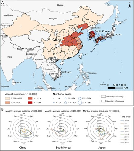
Table 1. Baseline demographic characteristics of reported SFTS patients in China, Japan and South Korea from 2010 to 2018.

	China	Japan	South Korea
No. of reported cases	11,995	396	866
Annual incidence (/10^5)	0.10	0.04	0.19
Average annual percent change (95% CI)	21.90% (−5.49%–49.29%)	12.20% (−20.06%–44.46%)	53.07% (2.30%–103.84%)
No. of deaths	881	107	173
Case fatality rate (%)	7.34	27.02	19.98
Age median (IQR)**	62 (52–70)	74 (5–96)	65 (64–66)
No. (%) of female cases	6375 (53.15%)	204 (51.52%)	436 (50.35%)
Major epidemic seasons	May–July	May–July	July, September–October
No. of affected provinces	25	23	17
Top 5 affected Provinces (total case number)
Top 1	Henan (3832)	Miyazaki (61)	Gyeonggi-do (146)
Top 2	Shandong (3466)	Kagoshima (39)	Gyeongsangbuk-do (136)
Top 3	Anhui (1833)	Yamaguchi (37)	Gangwon-do (125)
Top 4	Hubei (1566)	Hiroshima (35)	Gyeongsangnam-do (79)
Top 5	Liaoning (561)	Kochi (34)	Chungcheongnam-do (70)

Figure 2. Global recorded locations and model-predicted distribution probability of H. longicornis. (A) Each occurrence record of H. longicornis was geo-referenced and linked to the digital world map. The recording time of the H. longicornis presence was marked by colour gradients from red to green. (B) The potential geographic range of H. longicornis was predicted and mapped by using a maximum entropy method based on eco-geographical and climatic variables.

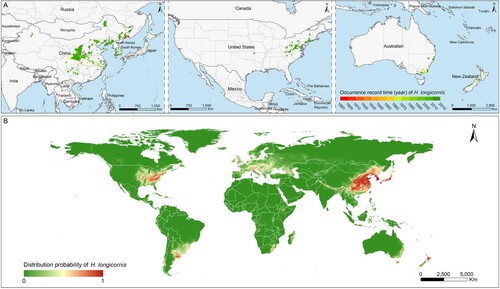
Table 2. The contribution of environmental variables to predict the global risk probability of H. longicornis presence based on ecological niche model.

Variable	Relative contribution
	Mean	Sd
Precipitation of warmest quarter (mm)	33.03	2.07
Annual average temperature (°C)	27.90	2.54
Population density (1 person/km^2)	19.68	3.57
Livestock density (1 head/km^2)	9.32	3.19
Mammalian richness (1 species/km^2)	2.89	0.84
Percentage of herbaceous vegetation of closed to open type (%)	1.98	0.63
Mean diurnal range of temperature (°C)	1.61	1.14
Rainfed croplands (%)	1.28	1.10
Elevation (m)	1.20	0.57
Percentage of broadleaved deciduous forest of closed type (%)	1.11	0.36

Figure 3. ROC curves for the risk probability of SFTS transmission based on climatic, eco-geographical and social variables by using BRT models. (A) The red curves are average predicted lines for risk factors by 100 repeats (grey lines) based on the bootstrapping procedure. (B) The grey lines are the ROC curve for 100 repeats, and the red, blue and black lines indicate the average ROC curves of 100 repeats based on the bootstrapping procedure for the train set, test set and prediction, respectively.

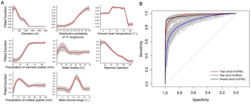
Table 3. The contribution of environmental variables to predict the occurrence of SFTS cases on the global range based on boosted regression trees model.

Variable	Relative contribution
	Mean	Sd
Elevation (m)	17.32	2.29
Predicted probability of H. longicornis presence	11.77	2.12
Annual mean temperature (°C)	11.58	1.49
Precipitation of warmest quarter (mm)	8.12	2.02
Water bodies (%)	6.75	1.81
Mammalian richness (1 species/km^2)	6.19	1.03
Precipitation of coldest quarter (mm)	5.57	1.63
Mean diurnal range of temperature (°C)	5.41	1.57
Irrigated croplands (%)	4.87	1.45
Precipitation of driest month (mm)	4.56	1.81
Other forests (%)	3.25	1.02
Livestock density (1 head/km^2)	2.65	0.74
Population density (1 person/km^2)	2.22	0.69
Needleleaved forests (%)	2.13	0.74
Broadleaved forests (%)	2.12	0.75
Build-up land (%)	1.95	0.57
Rainfed croplands (%)	1.92	0.50
Grassland (%)	1.62	0.46

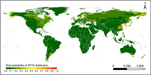
Figure 4. The potential distribution of human SFTS on global range based on BRT model. The probability of SFTS transmission was marked by different colour blocks.