
Figures & data
Table 1. Age and sex of QIV and ATIV cohorts.
Figure 1. Baseline antibody levels. In (A) individual profiles of HAI antibody responses at day 0 against Wt H1 and modified viruses H1-ΔSb, H1-ΔSa, H1-ΔCb and H1-ΔCa1 and H1-ΔCa2 is represented. GMT value is marked in each column. P-values were determined with the repeated measures one-way Bonferroni’s ANOVA for multiple comparisons test with the Geisser–Greenhouse correction; *P < .05, **P < .01, ***P < .001, ****P < .0001. In (B) SPR before vaccination was calculated as the percentage of patients that achieved HAI titres ≥ 1/40 for each virus and compared to the respective Wt H1 for each cohort. The two-tailed P-value was calculated with the McNemar’s test with the continuity correction; *P < .05, **P < .01, ***P < .001, ****P < .0001.
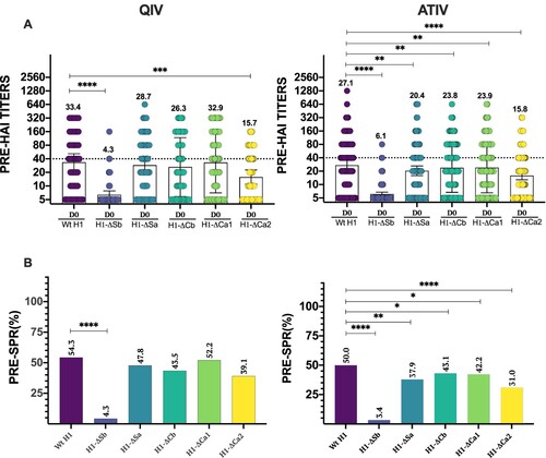
Figure 2. Response to vaccination. In (A) individual profiles of HAI antibody responses at day 28 against Wt H1 and modified viruses H1-ΔSb, H1-ΔSa, H1-ΔCb and H1-ΔCa1 and H1-ΔCa2 is represented. GMT value is marked in each column. P-values were determined with the repeated measures one-way Bonferroni’s ANOVA for multiple comparisons test with the Geisser–Greenhouse correction; *P < .05, **P < .01, ***P < .001, ****P < .0001. In (B) SPR after vaccination was calculated as the percentage of patients that achieved HAI titres ≥ 1/40 for each virus and compared to the respective Wt H1 for each cohort. The two-tailed P-value was calculated with the McNemar’s test with the continuity correction; *P < .05, **P < .01, ***P < .001, ****P < .0001. In (C) Fold induction of HAI titres or GMT increase (calculated as “GMTpost/GMTpre”) is represented of modified viruses H1-ΔSb, H1-ΔSa, H1-ΔCb and H1-ΔCa1 and H1-ΔCa2 compared to the Wt H1 in each cohort. P-values were determined with the repeated measures one-way Bonferroni’s ANOVA for multiple comparisons test with the Geisser–Greenhouse correction; *P < .05, **P < .01, ***P < .001, ****P < .0001. In (D) SCR was calculated as percentage of patients who reached a four-fold-induction for each virus and compared to its respective Wt H1 for each cohort. The two-tailed P-value was calculated with the McNemar’s test with the continuity correction; *P < .05, **P < .01, ***P < .001, ****P < .0001.
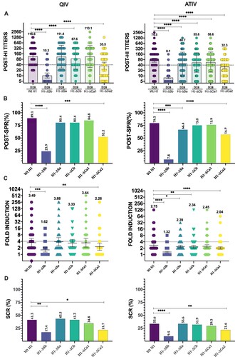
Table 2. Vaccination responses in the QIV and ATIV cohorts.
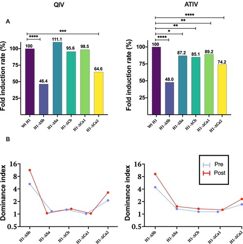
Figure 3. In (A) Fold Induction Rate ((FI mutant virus/FI Wt H1) × 100) of each virus is represented and compared to the Wt, which is 100%, in both cohorts. P-values were determined with the repeated measures one-way Bonferroni’s ANOVA for multiple comparisons test with the Geisser–Greenhouse correction; *P < .05, **P < .01, ***P < .001, ****P < .0001. In (B) Dominance index of HAI titres before and after vaccination with QIV and ATIV vaccines is represented.
Supplemental Material
Download MS Word (2 MB)Data availability statement
The data that support the findings of this study are available from the corresponding authors, T.A. and A.G-S. upon reasonable request.