Scheduling method of wind power generation for electricity market using state-of-charge transition and forecast error

Figures & data

Table 1. Outline of each market.

	Spot market	Intraday market
Time of market closure	10:00	1 h before
Start of creating generation schedules	9:30	1.5 h before
Time unit of a bid	30 min	30 min
Number of products	48	1

Figure 1. Production of generation schedules and adjustment of the actual output by using the ESS.

(a) One day before the target date: the generation schedules consisting of 48 products are produced for the spot market. Each product is based on the forecast data on the day before the target date. (b) One hour and a half before the ToD: the generation schedules for the intraday market are based on the new forecast data 1 h before the ToD. (c) ToD on the target date: the difference between the generation schedule and actual output is adjusted by using the ESS.

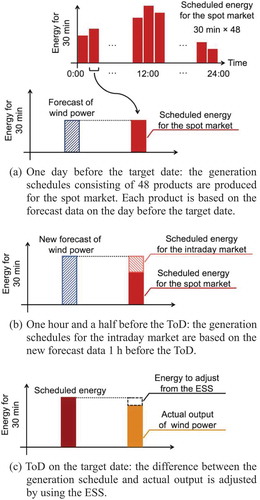
Table 2. Proposed scheduling methods.

	SOC transition	Forecast errors
Basic method	Not considered	Not considered
Method 1	Considered	Not considered
Method 2	Considered	Considered (Linear regression)
Method 3	Considered	Considered (Bagged trees)

Figure 2. Outline of the basic method.

(a) One day before the target date: the generation schedules consisting of 48 products are produced for the spot market. Each product is the same as the forecast data on the day before the target date. (b) One hour and a half before the ToD: the extra trade for the intraday market are the same as the difference between the generation schedule for the spot market and the new forecast data 1.5 h before the ToD.

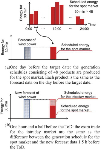
Figure 3. Outline of method 1.

(a) One day before the target date: SOC at 0:00 on the target date is estimated. The generation schedules for the spot market are designed by considering the SOC maintenance. (b) One hour and a half before the ToD: SOC at the ToD is estimated. The extra trade for the intraday market is produced by considering the SOC maintenance.

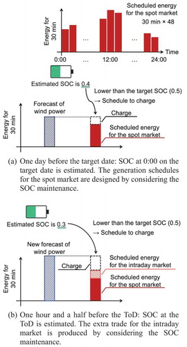
Figure 4. Outline of method 2.

(a) One day before the target date: SOC at 0:00 on the target date is estimated. The generation schedules for the spot market are produced by considering the SOC maintenance. (b.1) Error is estimated and forecast is adjusted with the linear regression model. (b.2) Generation schedule is designed using adjusted forecast. (b) One hour and a half before the ToD: the forecast error is estimated by using the model, and adjusted forecast data are calculated. SOC at the ToD is estimated, and the extra trade for the intraday market is produced by considering the SOC maintenance.

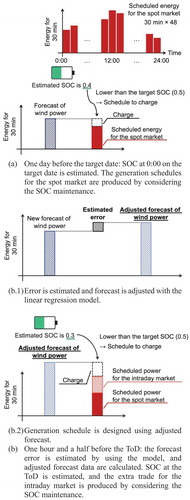
Table 3. Conditions for the linear regression model.

Predictor variable	Forecast errors at the current time
Response variable	Forecast error that appears in 1–119 min
Data for learning the model	Data from April 2012 to March 2013
Data for evaluation	Data from April 2012 to March 2013

Figure 5. Outline of method 3.

(a) One day before the target date: SOC at 0:00 on the target date is estimated. The generation schedules for the spot market are designed by considering the SOC maintenance (this step is the same as Fig. 4(a)). (b.1) Adjusted forecast considering errors is estimated with the bagged trees model. (b.2) Generation schedule is designed using adjusted forecast (this step is the same as Fig. 4(b.2)). (b) One hour and a half before the ToD: adjusted forecast data is estimated by using the model. SOC at the ToD is estimated, and the extra trade for the intraday market is designed by considering the SOC maintenance.

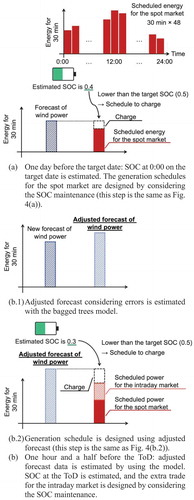
Table 4. Conditions for the bagged trees model.

Patterns of target time	Pattern 1: in 0–30 min Pattern 2: in 30–60 min Pattern 3: in 60–90 min Pattern 4: in 90–120 min
Predictor variable	Actual output at the current time Forecast data at the current time Forecast data in the target timing
Response variable	Adjusted forecast in the target timing
Data for learning the model	Data from April 2012 to March 2013
Data for evaluation	Data from April 2012 to March 2013
Cross-validation folds	5 folds
Minimum leaf size	8
Number of learners	30

Figure 6. Relationship between the predictor and response variables on each model.

(a) Linear regression model. (b) Bagged trees model.

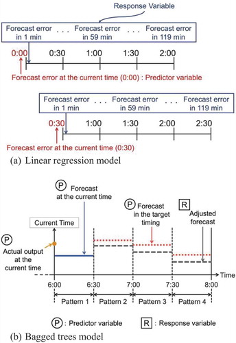
Figure 7. Coefficient obtained by the linear regression model.

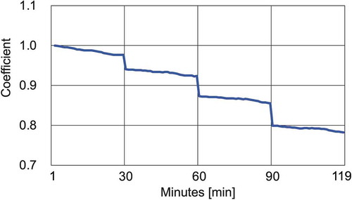
Table 5. Condition of the ESS.

Power [pu]	0.1, 0.2, 0.3, 0.4, 0.5
Hours to discharge [h]	3
Charge/discharge efficiency	Ratio is lower than 0.5: varies linearly from 0.9 to 0.95 Ratio exceeds 0.5: 0.95
Target SOC	0.5

Figure 8. Simulation outline.

Figure 9. Flow of the calculation in ToD (30 min).

Figure 10. Assumed system consisting of wind turbines and the ESS.

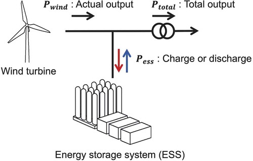
Figure 11. Histogram of SOC.

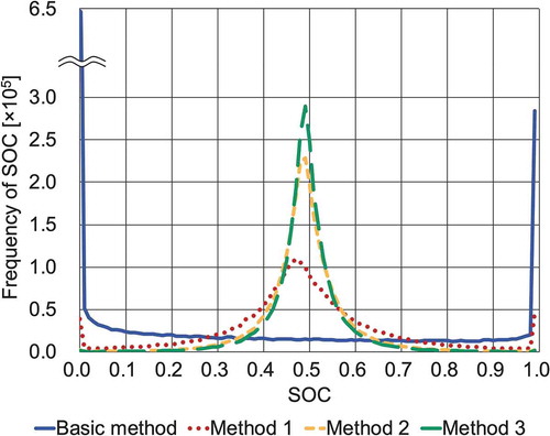
Table 6. Results of trades.

		Basic Method	Method 1	Method 2	Method 3
Spot market	Bid volume (sale) [pu-h]	2290.6	2286.3	2287.1	2287.3
Intraday market	Bid volume (sale) [pu-h]	247.5	325.9	391.4	374.2
	Bid volume (purchase) [pu-h]	−238.1	−342.4	−408.9	−389.4
Total bid volume [pu-h]		2300.0	2269.8	2269.5	2272.1
Imbalance [pu-h]		291.6	140.9	80.1	47.4
The ratio of the imbalance to total bid volume [%]		12.7	6.2	3.5	2.1

Figure 12. Imbalance between supplied energy and the generation schedules.

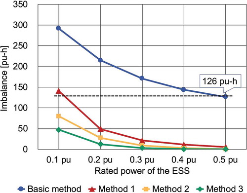
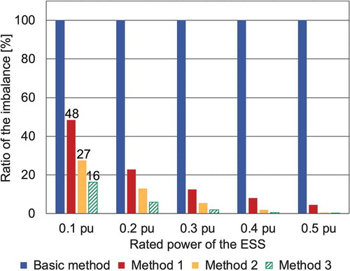
Figure 13. Ratio of the imbalance in each proposed method to that in the basic method.