Multi-sensor forest vegetation height mapping methods for Tanzania

Figures & data

Figure 1. Four Landsat images of the same area in Tanzania, all acquired in January but in different years: (a) 26 January 1987, (b) 21 January 1997, (c) 24 January 1998, (d) 14 January 2003. False colour images, with Landsat bands SWIR₂ (2220 nm), NIR (830 nm) and red (655 nm) shown as red, green and blue, respectively.

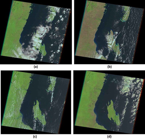
Table 1. Comparison of previous studies on forest canopy height estimation from remote sensing data.

Authors	Location	Tree species/forest type	Mean height [m]	Sensor	Grid [m]	R^2	RMSE [m]	RMSE [%]
Næsset (1997)	Hedmark, Norway	Pine, spruce	16.2	ALS	Stand	0.94	1.25	7.7%
Kwak et al. (2007)	South Korea	Pine, larch, oak	15.4	ALS	1	0.77	1.27	8.2%
Hopkinson et al. (2006)	Canada	Several forest types	17	ALS	1	0.95	1.80	10.6%
Véga and St-Onge (2008)	Quebec, Canada	Mixed managed forest	23.7	Aerial stereo pairs	0.5	0.96	1.09	4.6%
Lefsky et al. (2007)	Amazon	Tropical with dry season	17.2	ICESat GLAS	60	0.83	4.30	25.0%
	USA	Several forest types	18.9			0.73	5.01	26.5%
Lefsky (2010)	Globally	All forest types	15	ICESat GLAS + Modis	500	0.57	6.50	43.3%
Zhang et al. (2014)	California, USA	Several forest types	35	ICESat GLAS + Landsat	30	0.27	12.33	35.2%
Kellndorfer et al. (2004)	Georgia, USA	Pine plantation	17	SRTM	90	0.79	1.10	6.5%
	Sierra Nevada, USA	Mixed coniferous	17			0.74	4.60	27.1%
Kugler et al. (2014)	Krycklan, Sweden	Spruce and pine, occasional birch	18	TanDEM-X VV	12	0.91	1.58	8.8%
			18	TanDEM-X VV+HH		0.86	2.02	11.2%
	Traunstein, Germany	Spruce, beech, fir	27	TanDEM-X HH		0.8	3.30	12.2%
			27	TanDEM-X VV+HH		0.77	2.80	10.4%
	Mawas, Indonesia	Semi-deciduous peat swamp forest	16	TanDEM-X VV		0.95	1.90	11.9%
			16	TanDEM-X VV+HH		0.69	5.70	35.6%
Lei and Siqueira (2014)	Maine, USA	Several forest types	19.2	Palsar	400 × 800	0.34	3.60	18.8%
Sexton et al. (2009)	North Carolina, USA	Pine	28	ALS	6	0.83	2.22	7.9%
			28	GeoSAR	3	0.7	7.79	27.8%
			28	SRTM	30	0.54	13.42	47.9%
		Hardwood	25	GeoSAR	3	0.38	8.34	33.4%
			25	SRTM	30	0.35	16.39	65.6%
Helmer et al. (2010)	Bahamas	Tropical dry forest	3.5	Landsat time series	30	0.87	0.90	25.7%
Wilkes et al. (2015)	Victoria, Australia	Mixed	18	Landsat+Modis	30	0.58	5.68	31.3%
Wolter et al. (2009)	Minnesota, USA	Hardwood	16	SPOT-5	10	0.69	1.27	7.9%
		Coniferous	17			0.92	1.59	9.4%
Kalacska et al. (2007)	Costa Rica	Deciduous	12	Hyperion	30	0.92	1.10	9.2%
Chopping et al. (2009)	Colorado, USA	Several forest types	7	MISR	250	0.66	3.60	51.4%
Cartus et al. (2012)	Chile	Pine plantations	24	ALS	Stand	0.93	1.70	7.1%
			24	Palsar		0.72	2.75	11.5%
			24	Landsat		0.64	3.23	13.5%
			24	Landsat+Palsar		0.83	2.44	10.2%
Hyyppä et al. (2000)	Kalkkinen, Finland	Boreal	16.5	Airborne C-band SAR	Stand	0.77	2.97	18.0%
			16.5	Airborne hyperspetral		0.47	5.10	30.9%
			16.5	Aerial photograph		0.34	5.43	32.9%
			16.5	Spot multispectral		0.37	5.85	35.5%
			16.5	Landsat		0.26	6.05	36.7%
			16.5	ERS 1-day coherence		0.15	6.43	39.0%

Figure 2. The location and extent of the two study areas, shown on a map of Tanzanian district boundaries. The 100 km grid lines are in UTM zone 37 S.

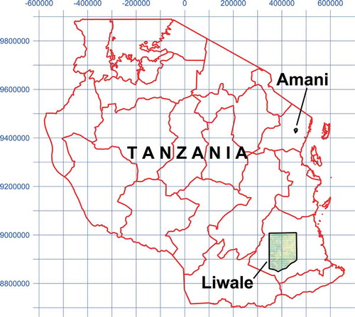
Table 2. Airborne laser scanning parameters.

	ALS campaign
	Amani 2012	Liwale 2012	Liwale 2014
Laser scanner	ALS70, snr 7160	ALS70, snr 7160	ALS70, snr 7204
Elevation over terrain	800 m	1200 m	1200 m
Flying speed	135 knots	150 knots	150 knots
Laser pulse frequency	339 200 Hz	193 200 Hz	193 200 Hz
Point density	10.6/m^2	1.8/m^2	1.8/m^2
Field of view	± 16 degrees	± 27.5 degrees	± 27.5 degrees
Acquisition dates	19 January–3 March	10 February–7 March	18 July–8 August
Strip width	459 m	1374 m	1374 m
Strip overlap	20%	N/A	N/A
Strip gaps	N/A	3626 m	3626 m

Figure 3. ALS normalized digital surface model (nDSM), i.e. vegetation height, for Liwale. The 25 km grid lines are in UTM zone 37 S.

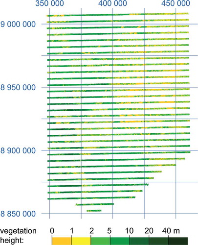
Figure 4. ALS normalized digital surface model (nDSM), i.e. vegetation height, for Amani. The 2 km grid lines are in UTM zone 37 S.

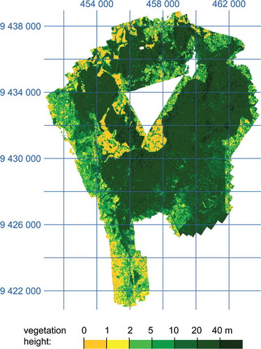
Table 3. Computation of scale factor for 2014 nDSM of ALS strips in Liwale.

Number of overlapping 30 m pixels	4,489,466
Mean 2012	5.219 m
Mean 2014	4.621 m
Mean difference	0.598 m
Scaling factor for 2014 nDSM	1.13

Table 4. Number of Landsat L1T acquisitions of path 166, rows 066–067 used in the study. On some dates, only one of the images (166/066 or 166/067) was available; in such cases, a sum of three numbers is shown. E.g., 3 + 1 + 2 means that three acquisitions of both 166/066 and 166/067 exist, then one of 166/066 only, and two of 166/067 only.

						Excluding SLC-off		Including SLC-off
Year	Landsat-4	Landsat-5	Landsat-7 SLC-on	Landsat-7 SLC-off	Landsat-8	Total L1T	Rejected L1G	Total L1T	Rejected L1G
1984		0 + 0 + 2				0 + 0 + 2	0 + 2 + 0
1985							1
1986		2 + 1 + 5				2 + 1 + 5	4 + 5 + 1
1987		0 + 0 + 1				0 + 0 + 1	2 + 2 + 0
1988	0 + 0 + 1					0 + 0 + 1	0 + 1 + 0
1989	1 + 0 + 1	0 + 0 + 1				1 + 0 + 2	0 + 1 + 1
1990		2 + 1 + 1				2 + 1 + 1	0 + 0 + 1
1991		3 + 0 + 1				3 + 0 + 1	2 + 1 + 0
1992		1				1
1993		4 + 0 + 2				4 + 0 + 2	0 + 1 + 0
1994		3 + 0 + 4				3 + 0 + 4	0 + 1 + 0
1995		3 + 0 + 2				3 + 0 + 2	5 + 2 + 1
1996		1 + 0 + 1				1 + 0 + 1	2 + 1 + 0
1997		3 + 0 + 4				3 + 0 + 4	4 + 3 + 0
1998		4 + 0 + 4				4 + 0 + 4	5 + 2 + 0
1999		2	3 + 1 + 1			5 + 1 + 1	1
2000		0 + 1 + 1	7 + 4 + 3			7 + 5 + 4	0 + 1 + 1
2001			8 + 4 + 2			8 + 4 + 2
2002			7 + 5 + 1			7 + 5 + 1
2003		1 + 0 + 1	4 + 1 + 0	1 + 3 + 1		6 + 4 + 2	0 + 0 + 1	6 + 4 + 2	1 + 0 + 2
2004		3 + 2 + 1		5 + 2 + 3		8 + 4 + 4	3 + 1 + 1	8 + 4 + 3	3 + 2 + 3
2005		2 + 0 + 1		7 + 2 + 5		9 + 2 + 6	2	9 + 2 + 6	2 + 2 + 2
2006		7 + 2 + 2		5 + 4 + 2		12 + 6 + 4	5 + 2 + 2	12 + 6 + 4	5 + 2 + 5
2007		2 + 2 + 0		6 + 2 + 2		8 + 4 + 2	3 + 0 + 2	8 + 4 + 2	3 + 0 + 5
2008		6 + 0 + 5		8 + 2 + 3		14 + 2 + 8	4 + 4 + 1	14 + 2 + 8	5 + 5 + 3
2009		5 + 0 + 1		8 + 5 + 3		13 + 5 + 4	1 + 1 + 0	13 + 5 + 4	1 + 2 + 6
2010		2 + 1 + 1		4 + 2 + 2		6 + 3 + 3	4 + 1 + 0	6 + 3 + 4	4 + 1 + 2
2011		2 + 1 + 0		5 + 3 + 1		7 + 4 + 1		7 + 4 + 1	1 + 0 + 3
2012				9 + 4 + 2				9 + 4 + 2	0 + 1 + 5
2013				8 + 6 + 2	13 + 2 + 0	13 + 2 + 0	0 + 0 + 1	21 + 8 + 2	4 + 1 + 7
2014				11 + 9 + 1	15 + 3 + 3	15 + 3 + 3	0 + 3 + 3	26 + 12 + 4	1 + 4 + 11

Figure 5. Landsat-8 data for Liwale for 20 January–6 December 2014, extracted from path 166, rows 066–067. False colour images with the same bands as in Figure 1. For six of the dates, either path/row 166/066 or 166/067 was not terrain corrected, and thus rejected, resulting in 15 complete extracts,3 partial extracts of the northern part (166/066), and 3 partial extracts of the southern part (166/067); this is indicated in Table 4 as 15 + 3 + 3 for Landsat-8 in 2014.

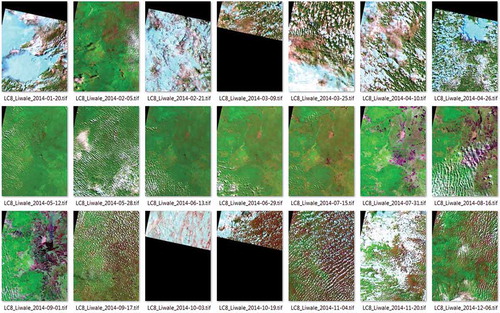
Figure 6. Mean vegetation height plotted for 0.1 SLAVI bins. Each curve is for one Landsat image, labelled “average-<day-number>”.

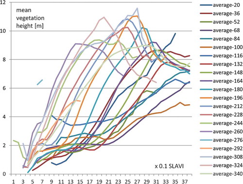
Figure 7. Scatterplot of SLAVI vs. ALS vegetation height for Landsat-8 data of 15 July 2014. Colour codes: white 0–1, Darkest blue 2, yellow 50, red 100, darkest red 140–1835. The solid black line is the same as the orange line labelled “average-196” in Figure 6, i.e. the mean vegetation height for any given 0.1 SLAVI bin. The dashed and dotted lines are the mean plus and minus one standard deviation, respectively.

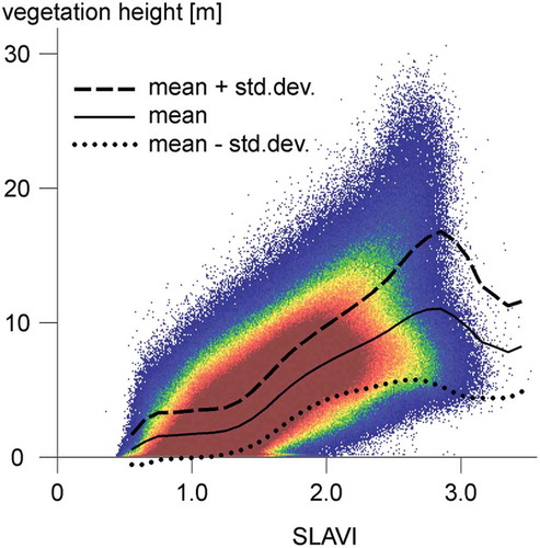
Table 5. Regressions between Landsat SLAVI and ALS vegetation height for Liwale, 2014. ¹Individual regressions for each Landsat image. ²Simultaneous regression with common constant but individual regression slopes.

			Separate regressions				Simultaneous regression
Date	Day	#cloud free	Regression constant^1 a	Regression slope^1 b	R^2	RMSE	Common constant^2 a0	Regression slope^2 b	R^2	RMSE
2014–01-20	20	83,274	−4.00	4.10	0.52	2.34	−3.40	3.80	0.52	2.35
2014–02-05	36	2,652,979	−4.71	4.86	0.44	3.22	−3.40	4.27	0.44	3.23
2014–02-21	52	0
2014–03-09	68	223,516	−2.20	2.10	0.23	2.32	−3.40	2.53	0.23	2.33
2014–03-25	84	161,719	−1.42	2.47	0.23	2.71	−3.40	3.24	0.23	2.75
2014–04-10	100	340,458	−0.49	1.68	0.07	3.16	−3.40	2.72	0.07	3.22
2014–04-26	116	389,276	0.84	1.84	0.08	3.58	−3.40	3.48	0.08	3.69
2014–05-12	132	3,597,385	−5.57	4.17	0.27	3.33	−3.40	3.33	0.27	3.34
2014–05-28	148	1,558,161	−4.95	4.32	0.33	3.08	−3.40	3.64	0.33	3.09
2014–06-13	164	3,954,445	−6.27	5.47	0.44	2.86	−3.40	4.11	0.44	2.91
2014–06-29	180	4,085,720	−5.92	6.12	0.48	2.89	−3.40	4.78	0.48	2.93
2014–07-15	196	4,430,895	−5.48	6.90	0.53	2.86	−3.40	5.65	0.53	2.90
2014–07-31	212	4,516,253	−3.98	6.78	0.49	3.01	−3.40	6.38	0.49	3.01
2014–08-16	228	3,432,935	−2.22	6.17	0.44	2.93	−3.40	7.08	0.44	2.96
2014–09-01	244	4,322,941	−1.96	7.25	0.34	3.29	−3.40	8.60	0.34	3.36
2014–09-17	260	1,821,464	−2.08	8.85	0.24	3.52	−3.40	10.37	0.24	3.60
2014–10-03	276	0
2014–10-19	292	331,082	−0.32	3.82	0.09	1.70	−3.40	8.03	0.09	1.81
2014–11-04	308	1,905,920	−0.81	6.70	0.26	3.69	−3.40	9.19	0.26	3.80
2014–11-20	324	504,222	−2.72	8.19	0.36	3.51	−3.40	8.82	0.36	3.61
2014–12-06	340	2,433,464	−1.23	4.65	0.36	3.51	−3.40	5.95	0.36	3.75

Figure 8. The two alternative regression lines for 15 July 2014 superimposed on the scatter plot.

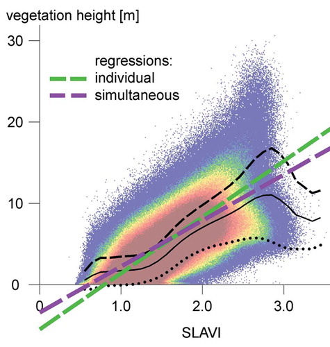
Table 6. Dependent and independent variances of vegetation height estimated from repeated Landsat acquisitions.

Total number of observations, N	41 466 327
Number of ALS measurements, I	4 599 924
Total variance, τ^2+σ^2	10.26 m^2
Dependent variance, σ^2	8.05 m^2
Independent variance, τ^2	2.21 m^2
Mean value of mean vegetation height estimated from 21 Landsat images	5.36 m
Mean value of ALS measured mean vegetation height	5.23 m
Deviation of mean	0.13 m

Figure 9. PALSAR backscatter versus ALS vegetation height. Exponential regression lines (solid lines) were fitted to the data points (cyan symbols for HV and purple symbols for HH polarization).

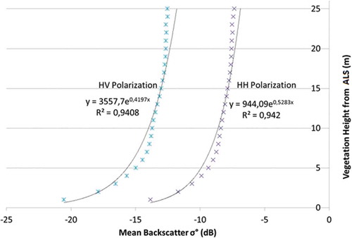
Table 7. PALSAR estimates of vegetation height for 2007–2010 versus ALS measurements for 2012.

	2007	2008	2009	2010	Average
Mean ALS vegt. height 2012					5.203 m
Mean PALSAR vegt. height	5.804 m	5.718 m	5.340 m	5.311 m	5.543 m
PALSAR deviation of mean	0.601 m	0.515 m	0.137 m	0.109 m	0.818 m
Kalman gain factor	1.115	1.099	1.026	1.021	1.065
Variance	10.301 m^2	8.222 m^2	7.785 m^2	7.629 m^2	8.484 m^2

Table 8. Average vegetation height estimates for Liwale. Landsat data includes all Landsat-4, 5, 7 and 8 data (Landsat 7 SLC-off data is also included).

Satellite estimate	ALS data	# valid pixels	Satellite mean	ALS nDSM mean	Deviation of mean	R^2	RMSE	RMSE %
Landsat 7, 2012	2012	4,553,483	5.344 m	5.211 m	0.133 m	0.46	2.91 m	55.8
Landsat Kalman (1984) 2012	2012	4,586,329	5.332 m	5.203 m	0.119 m	0.51	2.81 m	54.0
Landsat + PALSAR, Kalman (1984) 2012	2012	4,586,309	5.327 m	5.203 m	0.123 m	0.53	2.74 m	52.7
Landsat 7 + 8, 2014	2014	4,636,822	5.309 m	5.234 m	0.086 m	0.51	3.03 m	58.0
Landsat Kalman (1984) 2014	2014	4,642,954	5.305 m	5.221 m	0.083 m	0.54	2.98 m	57.0
Landsat + PALSAR, Kalman (1984) 2014	2014	4,639,257	5.305 m	5.219 m	0.085 m	0.55	2.97 m	56.9

Figure 10. Estimated mean vegetation height for ALS area in Liwale.

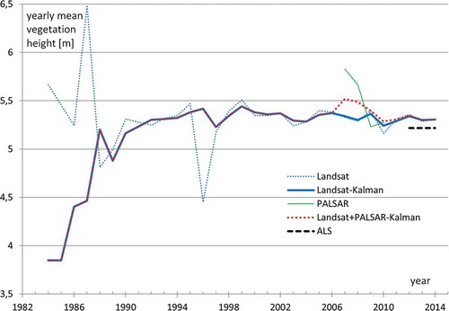
Figure 11. Change maps for a 7 km × 7 km area in Liwale. Red = reduction in vegetation height, blue = increase in vegetation height, white = unchanged. (a) ALS 2012–2014, up to 13.7 m reduced average height (darkest red) was measured within 30 m × 30 m pixels. The largest increase was 2.7 m (darkest blue). Black is no data. (b) Difference for 2012–2014 estimated from Kalman filtered multi-sensor time series, differences range from −8.6 to 5.2.

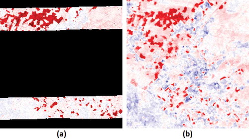
Table 9. Average vegetation height estimates for Amani.

Satellite estimate	ALS data	# valid pixels	Satellite mean	ALS nDSM mean	Deviation of mean	R^2	RMSE	RMSE %
Landsat 7, 2012	2012	129,975	12.26 m	18.91 m	6.647 m	0.29	13.43 m	71.0
Kalman filtered Landsat (1984) 2012	2012	136,789	12.15 m	19.07 m	6.922 m	0.34	13.57 m	71.2

Figure 12. Result of using the method on the Amani area. Grey values are scaled from 0 m (black) to 20 m (white), except for the difference image (d), which is scaled from −20 m (black) to 20 m (white). Areas outside of ALS coverage are set to 0 m. (a) Estimated vegetation height for 2012 from Landsat-7. Actual values range from 0 to 24 m. (b) Estimated vegetation height for 2012 from Landsat time series 1984–2012 with Kalman filtering. Actual values: 0–20 m. (c) ALS nDSM, actual values: 0–60 m. (d) Difference of estimates from Landsat with Kalman filtering and ALS, i.e. (b) minus (c). Actual values: −40 m to +25 m.

Næsset, E. (1997). Determination of mean tree height of forest stands using airborne laser scanner data. ISPRS Journal of Photogrammetry & Remote Sensing, 52, 49–56.

 Web of Science ®Google Scholar

Kwak, D.-A., Lee, W.-K., Lee, J.-H., Biging, G.S., & Gong, P. (2007). Detection of individual trees and estimation of tree height using LiDAR data. Journal of Forest Research, 12, 425–434.

 Web of Science ®Google Scholar

Hopkinson, C., Chasmer, L., Lim, K., Treitz, P., & Creed, I. (2006). Towards a universal lidar canopy height indicator. Canadian Journal of Remote Sensing, 32(2), 139–152.

 Web of Science ®Google Scholar

Véga, C., & St-Onge, B. (2008). Height growth reconstruction of a boreal forest canopy over a period of 58 years using a combination of photogrammetric and lidar models. Remote Sensing of Environment, 112, 1784–1794.

 Web of Science ®Google Scholar

Lefsky, M.A., Keller, M., Pang, Y., Camargo, P.B., & Hunter, M.O. (2007). Revised method for forest canopy height estimation from Geoscience Laser Altimeter System waveforms. Journal of Applied Remote Sensing, 1, 013537.

 Web of Science ®Google Scholar

Lefsky, M.A. (2010). A global forest canopy height map from the moderate resolution imaging spectroradiometer and the geoscience laser altimeter system. Geophysical Research Letters, 37, L15401. doi:10.1029/2010GL043622

 Web of Science ®Google Scholar

Zhang, G., Ganguly, S., Nemani, R.R., White, M.A., Milesi, C., Hashimoto, H., … Myneni, R.B. (2014). Estimation of forest aboveground biomass in California using canopy height and leaf area index estimated from satellite data. Remote Sensing of Environment, 151, 44–56.

 Web of Science ®Google Scholar

Kellndorfer, J., Walker, W., Pierce, L., Dobson, C., Fites, J.A., Hunsaker, C., … Clutter, M. (2004). Vegetation height estimation from Shuttle Radar Topography Mission and National Elevation Datasets. Remote Sensing of Environment, 93, 339–358.

 Web of Science ®Google Scholar

Kugler, F., Schulze, D., Hajnsek, I., Pretzsch, H., & Papathanassiou, K.P. (2014). TanDEM-X pol-inSAR performance for forest height estimation. IEEE Transactions on Geoscience and Remote Sensing, 52(10), 6404–6422.

 Web of Science ®Google Scholar

Lei, Y., & Siqueira, P. (2014). Estimation of forest height using spaceborne repeat-pass L-band InSAR correlation magnitude over the US state of Maine. Remote Sensing, 6, 10252–10285.

 Google Scholar

Sexton, J.O., Bax, T., Siqueira, P., Swenson, J.J., & Hensley, S. (2009). A comparison of lidar, radar, and field measurements of canopy height in pine and hardwood forests of southeastern North America. Forest Ecology and Management, 257, 1136–1147.

 Web of Science ®Google Scholar

Helmer, E.H., Ruzycki, T.S., Wunderle, J.M., Jr., Vogesser, S., Ruefenacht, B., Kwit, C., … Ewert, D.N. (2010). Mapping tropical dry forest height, foliage height profiles and disturbance type and age with a time series of cloud-cleared Landsat and ALI image mosaics to characterize avian habitat. Remote Sensing of Environment, 114, 2457–2473.

 Web of Science ®Google Scholar

Wilkes, P., Jones, S.D., Suarez, L., Mellor, A., Woodgate, W., Soto-Berelov, M., … Skidmore, A. (2015). Mapping forest canopy height across large areas by upscaling ALS estimates with freely available satellite data. Remote Sensing, 7, 12563–12587.

 Google Scholar

Wolter, P.T., Townsend, P.A., & Sturtevant, B.R. (2009). Estimation of forest structural parameters using 5 and 10 meter SPOT-5 satellite data. Remote Sensing of Environment, 113, 2019–2036.

 Web of Science ®Google Scholar

Kalacska, M., Sanchez-Azofeifa, G.A., Rivard, B., Caelli, T., White, H.P., & Calvo-Alvarado, J.C. (2007). Ecological fingerprinting of ecosystem succession: Estimating secondary tropical dry forest structure and diversity using imaging spectroscopy. Remote Sensing of Environment, 108, 82–96.

 Web of Science ®Google Scholar

Chopping, M., Nolin, A., Moisen, G.G., Martonchik, J.V., & Bull, M. (2009). Forest canopy height from the Multiangle Imaging SpectroRadiometer (MISR) assessed with high resolution discrete return lidar. Remote Sensing of Environment, 113, 2172–2185.

 Web of Science ®Google Scholar

Cartus, O., Kellndorfer, J., Rombach, M., & Walker, W. (2012). Mapping canopy height and growing stock volume using airborne lidar, ALOS PALSAR and Landsat ETM+. Remote Sensing, 4, 3320–3345.

 Google Scholar

Hyyppä, J., Hyyppä, H., Inkinen, M., Engdahl, M., Linko, S., & Zhu, Y.-H. (2000). Accuracy comparison of various remote sensing data sources in the retrieval of forest stand attributes. Forest Ecology and Management, 128, 109–120.

 Web of Science ®Google Scholar