Mapping ultramafic complexes using airborne imaging spectroscopy and spaceborne data in Arctic regions with abundant lichen cover, a case study from the Niaqornarssuit complex in South West Greenland

Figures & data

Figure 1. General 1:500 000 geological map across the southern Nagssugtoqidian Orogen simplified from Garde and Marker (2010). The location of number of mafic and ultramafic complexes mapped by processing of regional HyMAP data are shown in pink ovals. The Niaqornarssuit complex is highlighted by a black oval

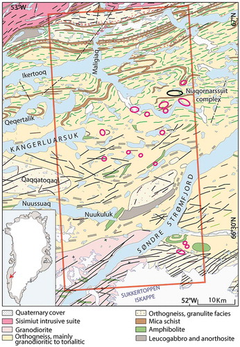
Figure 2. View of the Niaqornarssuit complex, highlighting characteristic features of the study area terrane (e.g. variability in spatial continuity of exposed outcrop, lichen coatings, and low-lying vegetation cover)

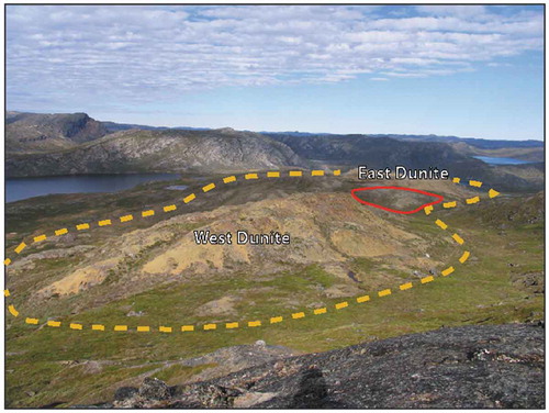
Figure 3. True color HyMAP image and detailed geological map of the Niaqornarssuit complex produced by 21^st North Exploration Company. Yellow dots show the locations of surface samples that have been collected for reconnaissance work and mapping over the area. Samples that are selected for XRF and ASD analysis are indicated by red color

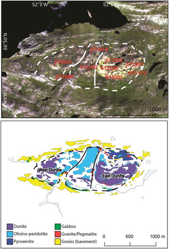
Figure 4. (a) Field localities where spectroradiometric measurements were carried out. The area covered by the airborne hyperspectral survey is indicated by the red line. K = kimberlitic rocks, L = lamproitic rocks, LG = local geology, S = rocks of the Sarfartoq carbonatite complex, P = pseudo-invariant fields, Plant = vegetation; (b) locality P3 on the silt formation in the vicinity of Kangerlussuaq airport; (c) individual measurements from the locality P3

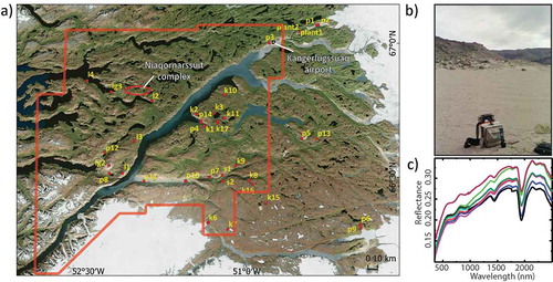
Figure 5. Airborne HyMAP data before and after removal of remaining albedo differences using detrending approach

Table 1. Mafic and ultramafic samples and mineralogical composition determined from X-ray fluorescence analysis (hornblende: hnb, pyroxene: px, olivine: ol, serpentine: srp)

Sample nr.		SiO2	TiO2	Al2O3	FeO	Fe2O3	MnO	MgO	CaO	Na2O	K2O	P2O5	H2O	CO2	LOI	SO3
		(%)	(%)	(%)	(%)	(%)	(%)	(%)	(%)	(%)	(%)	(%)	(%)	(%)	(%)	(%)
671001	gabbro/amphibolite (hnb, px)	48.94	1.33	13.28	9.57	5.04	0.17	6.32	10.01	2.59	0.43	0.09	0.96	0.06	1.02
671003	peridotite/dunite	38.11	0.03	0.18	9.87	5.25	0.23	43.6	0.2	<0.01	<0.01	<0.01	0.32	0.22	0.55
671004	metagabbro (hnb, px)	47.34	1.45	14.19	8.97	5.08	0.22	7.4	9.5	2.14	0.59	0.17	1.36	0.25	1.61
671006	gabbro	49.28	2.23	12.73	9.62	5.64	0.25	5.04	7.47	0.97	2.12	0.19	1.82	1.13	2.95
671014	peridotite (ol, ± px)	40.52	0.21	2.24	7.05	4.67	0.25	36.91	3.22	<0.01	<0.01	<0.01	3.45	0.16	3.62
671015	dunite (ol exclusively)	40.28	0.02	0.07	6.21	3.02	0.15	49.08	0.15	<0.01	<0.01	<0.01	0.05	0.13	0.18
671022	peridotite	51.69	0.19	1.47	3.75	4.88	0.17	19.23	16.23	<0.01	0.07	<0.01	1.49	0.11	1.6
671023	pyroxenite	50.09	0.05	0.45	6.93	2.21	0.1	38.12	0.1	<0.01	0.06	0.02	0.79	0.31	1.09
671034	amphibolite	35.31	1.99	3.9	10.49	8.83	0.2	24.13	3.43	<0.01	0.04	0.16	7.31	2.78	10.08
671038	amphibolite	89.63	0.02	<0.01	4.08	4.11	<0.01	0.15	0.04	<0.01	<0.01	<0.01	0.01	0.15	0.16	4.36
671251	peridotite (ol, px)	23.87	0.03	0.06	10.79	21.58	0.1	18.47	0.83	<0.01	<0.01	<0.01	8.49	0.13	8.61	8.69
671254	peridotite/pyroxenite	40.73	0.03	0.13	7.82	4.38	0.32	44.1	0.13	<0.01	0.12	<0.01	0.16	0.16	0.32	0.41
671255	dunite/peridotite	56.69	0.02	0.25	8.34	0.96	0.28	28.24	0.68	<0.01	0.07	0.02	2.5	0.52	3.02
671260	pyroxenite (px, srp)	48.5	0.04	1.26	8.43	1.11	0.24	37.79	0.27	<0.01	0.01	<0.01	0.82	0.29	1.11
671265	peridotite/pyroxenite	34.42	0.04	0.12	13.31	6.95	0.2	36.18	1.25	<0.01	<0.01	0.01	1.45	0.23	1.68	4.63
671268	pyroxenite/peridotite	35.29	0.05	0.11	10.16	11.05	0.21	34.74	1.88	<0.01	<0.01	0.01	0.94	0.18	1.11	1.72
671357	peridotite (ol, px)	32.43	0.1	0.78	8.06	16.29	0.23	32.78	1.47	<0.01	0.05	0.01	1.8	0.07	1.87	1.37
671372	peridotite (ol, px)	38.3	0.03	0.23	7	8.32	0.25	43.88	0.02	<0.01	<0.01	<0.01	0.32	0.08	0.4

Figure 6. Schematic representation of the workflow for ISMA and EnGeoMAP mapping methods

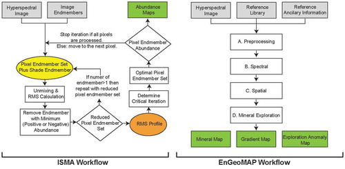
Figure 7. Spectral end-members used for ISMA and EnGeoMAP mapping methods. Outcrop related endmembers using (a) full range of spectral bands and (b) knowledge-based band selection. Vegetation and lichen related endmembers using (c) full range of spectral bands and (d) knowledge-based band selection. See Table 2 for detailed description of the selected spectral bands

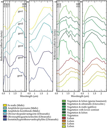
Figure 8. Comparison of HyMAP endmembers (solid lines) derived from SSEE with best matches from laboratory sample average spectra and mineral spectra taken from the USGS spectral library for (a,b) gabbro, (c,d) pyroxenite, (e,f) peridotite and (g,h) dunite samples. See Table 1 for detailed description of mineralogical composition of each sample determined from X-ray fluorescence analysis

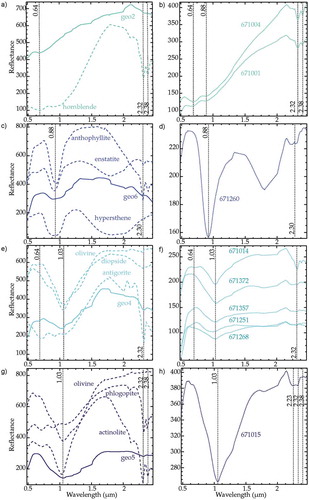
Table 2. Spectral bands used for SSEE and ISMA, wavelength in µm

VNIR	0.562, 0.571, 0.586, 0.617, 0.633, 0.648, 0.663, 0.678, 0.740, 0.785, 0.888, 0.936, 1.030, 1.076, 1.091, 1.279
SWIR	1.658, 1.670, 1.732, 2.098, 2.116, 2.204, 2.220, 2.257, 2.274, 2.308, 2.324, 2.340, 2.357, 2.373, 2.389, 2.405

Figure 9. (a) HyMAP continuum removed RGB color composite highlighting the main mafic-ultramafic units. Red – ferric iron (0.64 μm); Green – Mg-OH (2.32 μm); and Blue – ferrous iron (1.03 μm). (b) False-colour composite image highlighting the abundance of vegetation in the area. Classification results for HyMAP data generated from (c) ISMA, (d) best fit and (e) BVLS methods

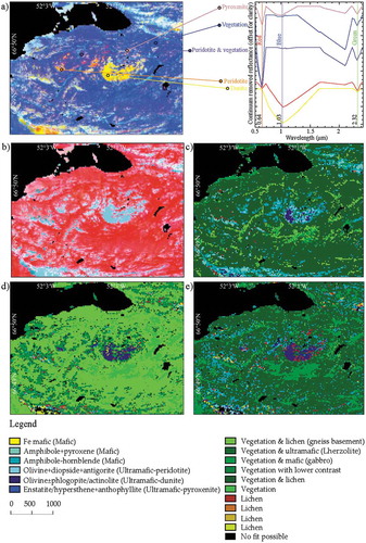
Figure 10. Spectral unmixing results from ISMA and EnGeoMAP showing abundances for (a,g) geo2 – mafic (amphibole + pyroxene); (b,h) geo3 – mafic (amphibole – hornblende); (c,i) geo4 – peridotite (olivine + diopside + antigorite); (d,j) geo5 – dunite (olivine ± phlogopite/actinolite); and (e,k) geo6 – pyroxenite (enstatite/hypersthene + anthophyllite) endmembers. RGB color composites of abundances for (f) ISMA and (l) EnGeoMAP highlighting the main mafic-ultramafic units. Red – mafic (geo2); Green – peridotite; and Blue – dunite

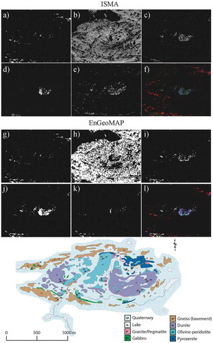
Figure 11. Classification results generated from BVLS for simulated ASTER, Landsat-8 OLI, and Sentinel-2. HyMAP BVLS and ISMA data are used as a reference base and similarity scores for each endmember and sensor to the HyMAP reference are indicated in the plot

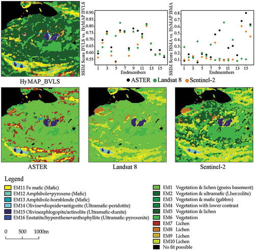
Table 3. Quantitative comparison between the results generated using different processing approaches with the reference image

Figure 12. a) The binarized dunite class from the geological map is used as ground truth. The binarized classification results for HyMAP data generated using b) ISMA, c) best fit, and d) BVLS methods for the dunite endmember

Garde, A. A. , & Marker, M. (2010). Geological map of Greenland, 1:500 000, Søndre Strømfjord – Nuussuaq, Sheet 1 (2nd ed.). In n. edition (Ed.). Geological Survey of Denmark and Greenland.

 Google Scholar