
Figures & data
Figure 1. Spatial extent of the study area showing a part of Kottayam and Alappuzha districts in Kerala, India
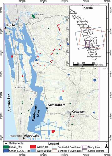
Figure 2. Methodology showing flood area mapping using EO images
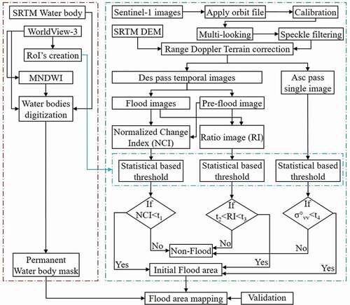
Figure 3. The sub-figures (a) show the PWB mask obtained by the proposed approach and (b) shows the PWB mask obtained by the JRC GSW layer. The sub-figure (c) shows the random points overlaid on the PWB obtained by the proposed approach
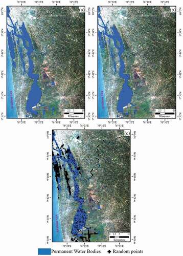
Figure 4. Statistical analysis of water, urban and other land use classes ROIs obtained from temporal indices (a) NCI and (b) RI
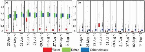
Figure 5. Change detection-based flood area plotted against IMD rainfall
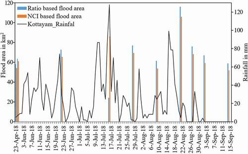
Figure 6. Change detection based flood maps obtained from pre-flood images. The figures (a), (b), (c) are the enlarged part of the rectangles shown in the left figures, but with SAR image as background. The rectangles are overlaid on Sentinel-2 true colour image on the top row and Open Street MAP (OSM) at the other rows
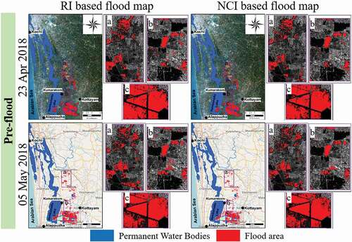
Figure 7. Change detection based flood maps obtained with pre-flood and during flood images. The figures (a), (b), (c) are the enlarged part of the rectangles shown in the left figures, but with SAR image as background. The rectangles are overlaid on Sentinel-2 true colour image on the top row and Open Street MAP (OSM) at the other rows
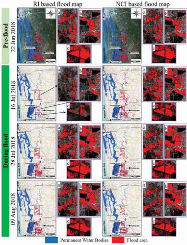
Figure 8. Change detection based flood maps obtained with during flood and post-flood images. The figures (a), (b), (c) are the enlarged part of the rectangles shown in the left figures, but with SAR image as background. The rectangles are overlaid on Sentinel-2 true colour image on the top row and Open Street MAP (OSM) at the other rows
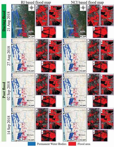
Figure 9. Flood area extracted from a single SAR image using the threshold method. The figures (a) and (c) are characterized mostly by agricultural land uses. Figure (b) is characterized by mixed land uses (buildings, roads, trees, open areas). The rectangles are overlaid on Sentinel-2 true colour image
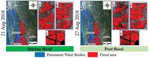
Figure 10. Temporal dynamics of land surface condition for a zoomed-in portion (b). Pre, During and Post indicated the images acquired on pre-flood, during flood, and post-flood. Plot-1 and Plot-2 show the agricultural areas
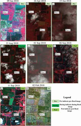
Figure 11. Flood area (excluding common area) extracted from both ascending and NCI images. The figures (a), (b), (c) are the enlarged part of the rectangles shown in the left figures. The rectangles are overlaid on Open Street MAP (OSM) layer
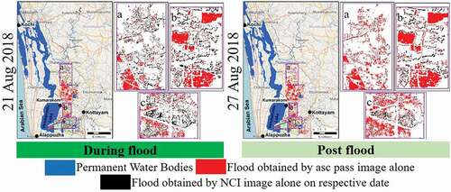
Figure 12.. (a), (b), (c), (d) shows an aerial view that has partially submerged houses on a flooded area located in and around Alappuzha and Kottayam districts
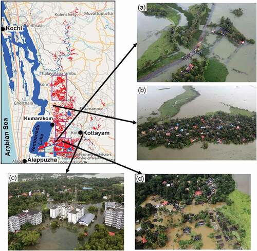
Table 1. EO satellite images used for Kerala flood mapping occurred in 2018