A method for in-field railhead crack detection using digital image correlation

Figures & data

Table 1. Simulation parameters, see also Figure 1 for the definitions of lengths.

Parameter	Value
Elastic modulus of ground	150 MPa
Poissons ratio of ground	0.3
Depth of ground under sleeper	2.0 m
Ground thickness (plane strain)	0.5 m
Sleeper dimension along track	0.25 m
Sleeper spacing	0.65 m
Spring stiffness of rail pad	120 kN/mm
Rail elastic modulus	210 GPa
Rail moment of inertia	2074 cm^4
Total rail length (free ends)	65.0 m
Wheel spacing, $L_{\mathrm{w}\mathrm{h}}$	1.8 m
Bogie spacing, $L_{\mathrm{b}}$	8.8 m
Waggon spacing, $L_{\mathrm{w}\mathrm{a}}$	13.8 m
Load from each wheel	122.6 kN

Figure 1. Rail deflection and bending moment due to a train passage. Camera A measures the undeformed rail surface while Camera B measures the deformed surface. The dimensions $L_{\mathrm{w}\mathrm{h}}$, $L_{\mathrm{b}}$, and $L_{\mathrm{w}\mathrm{a}}$ are described in Table 1, and $L_{\mathrm{c}}$ is the distance from the wheel to Camera B.

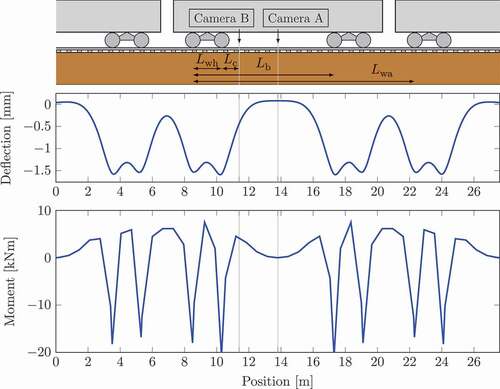
Figure 2. Illustration of the measured strain around a crack mouth in a rail subjected to a positive bending moment.

Figure 3. DIC experimental setup with the yellow hydraulic cylinders exerting a 4-point bending in the rail samples.

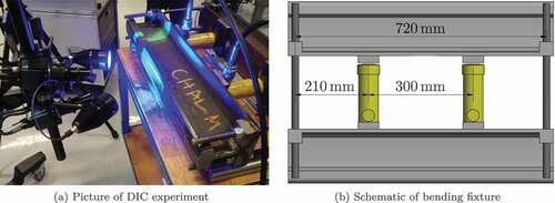
Figure 4. Surface strain distribution along the rail (horizontal in this figure), measured by DIC.

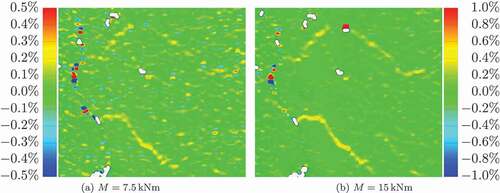
Figure 5. The extracted sample used to characterize the crack networks.

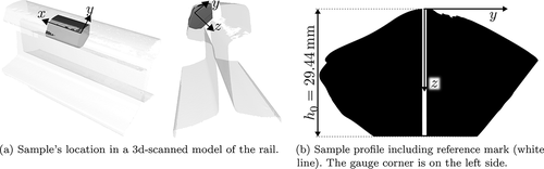
Figure 6. Example of conversion from optical microscopy images to binary images. The shown images are $1.5\mathrm{m}\mathrm{m}\times 1.5\mathrm{m}\mathrm{m}$.

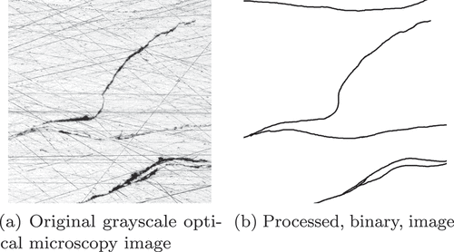
Figure 7. DIC results, viewed from above the microscopy sections. The black rectangle at $x=y=0$ shows the location of the reference mark, and axes correspond to the axes in .Figure 9 with dimensions in mm. The same strain scale as in Figure 4(b) is used. The coloured circles show the end-points of the cracks marked with the corresponding translucent colour in Figure 9

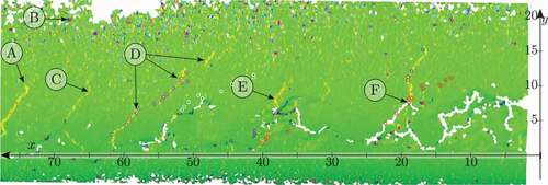
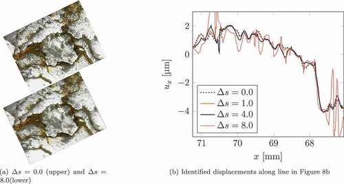
Figure 8. 2D DIC displacement identification based on the natural speckle pattern.

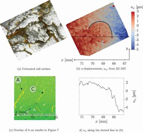
Figure 9. Sections showing the crack patterns with inverted colours compared to Figure 6. All coordinates are in mm. The horizontal lines have 5 mm spacing, the numbers next to the positive and negative y-axes denote the respective axis’ length, and the $z$-coordinate is defined in Figure 5(b). The translucent colours show how different cracks evolve between the sections and their top endpoints are marked by circles of the corresponding colour in Figure 7

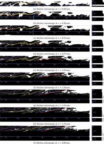
Figure 9. Continued.

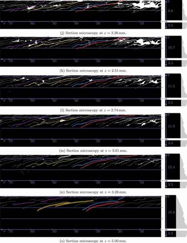
Figure 10. Correlation between cracks and DIC surface strains at $z=-1.51\mathrm{m}\mathrm{m}$. More sections are available in the supplementary material ‘CracksToDIC_Correlation.pdf’.

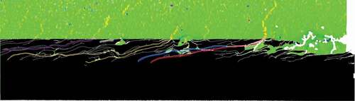
Figure 11. Moment variation beneath cameras during rolling. (a) shows the moment variation for the position of Camera B indicated by the black circle in (b).

Figure 12. Dimensions of the crack in the finite element model.

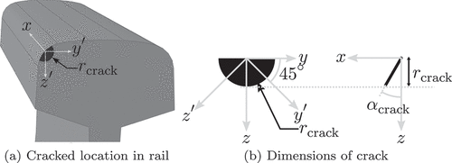
Figure 13. Longitudinal strain for a 5 mm deep crack with ${\alpha }_{\mathrm{c}\mathrm{r}\mathrm{a}\mathrm{c}\mathrm{k}}={45}^{\circ }$. Displacements are amplified 50 times.

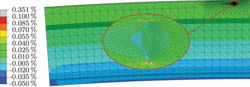
Figure 14. FE-modelling results.

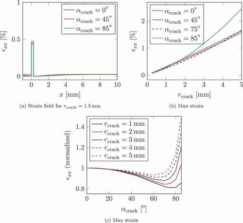
Figure 15. Custom lens (red) to capture the compressive strains close to the wheel.

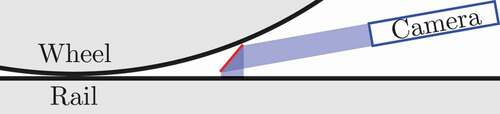
Figure 16. The motion blur effect.