Figures & data
Figure 1. A schematic representation of the model discussed in this paper. The platoon forming algorithms in this paper determine how the platoons are constructed. In the next step, a speed profiling algorithm determines how each individual vehicle approaches the intersection. Figure (a,b) corresponds, respectively, to the situation in (c) at times t = 4 and t = 8 seconds.
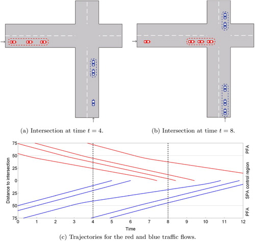
Figure 2. Algorithm 4 (solid lines) and Algorithm 5 (dashed lines) for several vehicles with t (s) on the horizontal axis and (m) on the vertical axis for several vehicles.
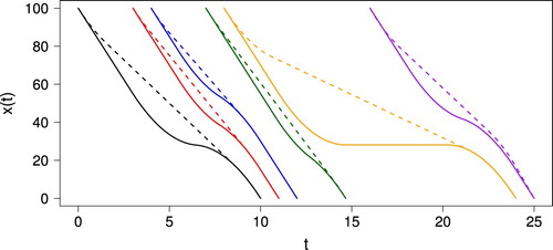
Figure 3. Three sample trajectories with one full stop. The optimal trajectory is plotted in solid black. The dashed green trajectory has a smaller value of compared to the optimal trajectory, whereas the dotted red trajectory has a smaller value of
.
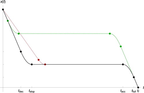
Figure 4. Visualization of the link between the traffic model with PFAs and polling models. The black line represents a self-driving vehicle, and the red dashed line represents the corresponding ‘vehicle’ in the vertical queueing model.
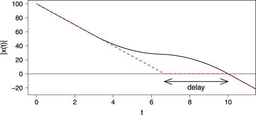
Figure 5. Mean delay experienced by an arbitrary car for the symmetric case (top) and asymmetric case (bottom). The solid and dashed lines represent simulation results and the dotted lines approximations.
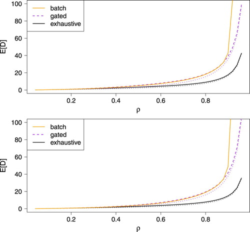
Figure 6. Fairness experienced by an arbitrary car for the symmetric case (top) and asymmetric case (bottom).
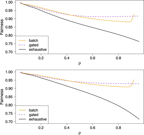
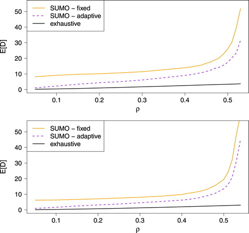
Figure 7. Mean delay for an arbitrary car for traditional traffic lights (represented by SUMO) and the exhaustive PFA for the symmetric example (top) and the asymmetric case (bottom).