A macroscopic flow model for mixed bicycle–car traffic

Figures & data

Figure 1. Sketch showing the numbering of the position x and spacing s for two platoons of cars and cyclists (a) and the linear interpolation to retrieve the car spacing at the positions of the bicycle platoons (b).

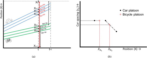
Figure 2. Single-class speed functions for cars and bicyclists.

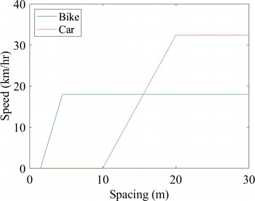
Table 1. Characteristic values used in the speed functions: jam spacing $s_{\mathrm{j}}$, critical spacing $s_{\mathrm{c}\mathrm{r}}$, free flow speed $v_{\mathrm{f}}$ and reduced speed $v_{\mathrm{r}\mathrm{e}\mathrm{d}}$

	$s_{\mathrm{j}}$ (m)	$s_{\mathrm{c}\mathrm{r}}$ (m)	$v_{\mathrm{f}}$ (m/s)	$v_{\mathrm{r}\mathrm{e}\mathrm{d}}$ (m/s)
cyclists	1.5	4.5	5.0	2.0
cars	5.0	10	9.0	-

Figure 3. Two-dimensional speed functions for cars (a) and bicyclists (b).

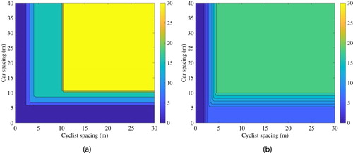
Figure 4. Simulation results for low demand situation ($s_b\left(t_0\right)=s_c\left(t_0\right)=20$ m), showing no speed adjustments when cars have a head start over cyclists (a) and cyclists have a head start over cars (b).

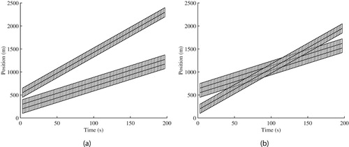
Figure 5. Simulation results for different demand situations. When initial spacings are $s_b\left(t_0\right)=10.2$ m and $s_c\left(t_0\right)=20$ m, cars can still overtake cyclists but at a reduced speed (a) and when initial spacings are $s_b\left(t_0\right)=10$ m and $s_c\left(t_0\right)=20$ m cars have to match the speed of cyclists (b). The magenta colouring appears when the speed is reduced and is more intense for lower speeds.

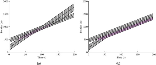
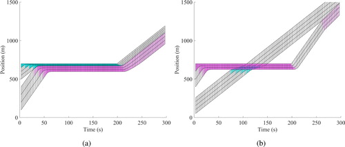
Figure 6. Simulation results for queuing situations. In (a) $s_b\left(t_0\right)=10.2$ m and $s_c\left(t_0\right)=20$ m and the cyclist have a head start of 450 m. In (b) $s_b\left(t_0\right)=10.4$ m and $s_c\left(t_0\right)=20$ m and the cars have a head start of 300 m. The cyan and magenta colouring appear when the speed is reduced for, respectively, cyclists and cars.