Stop-skipping in rolling horizons

Figures & data

Figure 1. Illustration of trips that we can modify their stop-skipping plans in two consecutive rolling horizons.

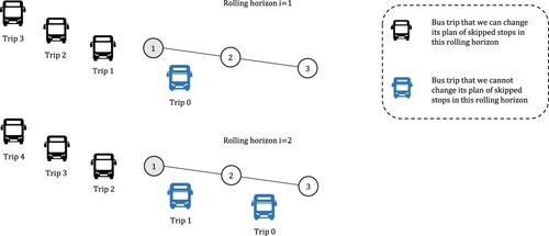
Figure 2. Required solution evaluations for a bus line with $|S|=20$ bus stops when the number of trips in the rolling horizon, $|N|$, varies. The possible computations are the computations that can be executed by the world's fastest supercomputer in 1 min.

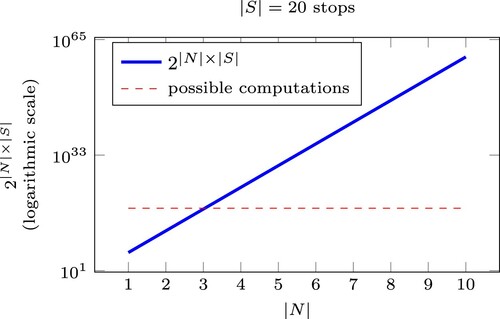
Figure 3. Required number of objective function evaluations with brute force and S-HC for rolling horizons with 1–10 trips, a bus line with 20 stops, and ${\mu }^{max}=5$.

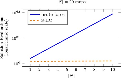
Figure 4. Topology of the toy network operating one bus line.

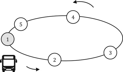
Table 1. Parameter values of the idealized scenario.

Parameter	Value	Parameter	Value
$r_1$	2 s	$c_1$	10 $/h
$r_2$	1 s	$c_2$	5 $/h
δ	20 s	$c_3$	7 $/h

Table 2. Computational costs and optimality gap(s) when applying Brute Force (BF), S-HC and the GA in the idealized bus line for different numbers of stops.

	Comput. Time (s)				Optimized $f\left(\mathbf{x}\right)$ ($)
Stops	BF	LINDO	S-HC	GA	BF	LINDO	S-HC	GA
3	0.11	0.19	0.96	1.03	169,101	169, 101	169,101	169,101
4	15.88	6.70	4.32	5.12	326,688	326,688	326,688	326,688
5	353.12	98.21	7.68	17.21	563,491	563, 491	563,491	595,819
6	−	259.19	21.62	41.89	−	897, 533	897,533	982,738

Figure 5. Convergence of the S-HC algorithm in the case of 5 bus stops and 4 trips in the rolling horizon.

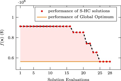
Figure 6. Computational cost when evaluating the performance of a single solution in a rolling horizon with 4 bus trips with respect to the number of stops.

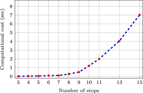
Figure 7. Stop-skipping candidates of bus line 15L in Denver.

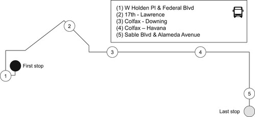
Table 3. Expected travel times, $\mathbb{E}\left[t_s\right]$.

origin$\to$destination	Travel time	origin$\to$destination	Travel time
1$\to$2	660 s	3$\to$4	1200 s
2$\to$3	660 s	4$\to$5	1080 s

Figure 8. Performance when applying the optimal stop-skipping solution in 1000 simulations considering $\mathrm{C}\mathrm{V}=0.2$, 0.3, 0.4, and 0.5, respectively.

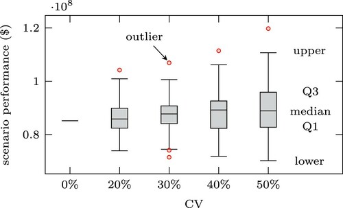
Table 4. Performance when running 1000 simulations for different travel time variation levels (in thousands).

CV	Minimum	Q1	Median	Q3	Maximum
0%	85,192	85,192	85,192	85,192	85,192
20%	73,947	82,426	85,845	89,908	100,917
30%	74,503	84,123	90,768	87,759	100,637
40%	71,864	82,373	89,220	92,630	106,184
50%	70,239	82,750	88,920	95,889	110,728

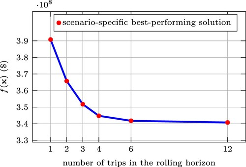
Figure 9. Performance of the stop-skipping strategy depending on the considered number of trips in a rolling horizon.