Figures & data
Figure 1. An example of a trial in dataset I. Participants were instructed to use right/left-hand motor imagery to move the cursor (the blue circle) to right/left toward the target (white circle). We considered movements toward/away from the target as good/bad movements perceived by the participants [Citation5].
![Figure 1. An example of a trial in dataset I. Participants were instructed to use right/left-hand motor imagery to move the cursor (the blue circle) to right/left toward the target (white circle). We considered movements toward/away from the target as good/bad movements perceived by the participants [Citation5].](/cms/asset/18fc860f-0e39-4b2d-b5b6-d5abb4614464/tbci_a_1671040_f0001_oc.jpg)
Figure 2. In dataset II, participants were instructed to ‘judge’ each cursor (red full circle) movement (indicated by the arrow in the static figure) as satisfactory or unsatisfactory with respect to its movement toward/away from the target (red empty circle) [Citation11]. Diagram (a) depicts a cursor’s location and diagrams (b) and (c) specify different next cursor movements and how the angle between the cursor direction of movement and the direct line connecting the cursor to the target location is defined. We considered angles smaller than 45° as good movements and larger than 130° as bad movements perceived by the participants.
![Figure 2. In dataset II, participants were instructed to ‘judge’ each cursor (red full circle) movement (indicated by the arrow in the static figure) as satisfactory or unsatisfactory with respect to its movement toward/away from the target (red empty circle) [Citation11]. Diagram (a) depicts a cursor’s location and diagrams (b) and (c) specify different next cursor movements and how the angle between the cursor direction of movement and the direct line connecting the cursor to the target location is defined. We considered angles smaller than 45° as good movements and larger than 130° as bad movements perceived by the participants.](/cms/asset/f4767365-0426-4a84-a22c-ca5f8b04866d/tbci_a_1671040_f0002_oc.jpg)
Figure 3. Method of CSP-CTP: CSP filters are trained on each frequency band ( and
). Six CSP filters (corresponding to the 3 largest and smallest eigenvalues) are selected and EEG epochs are filtered through each. Then, CTP filters are trained on the good (G) and bad (B) CSP-filtered data separately.
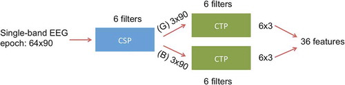
Figure 4. ERP in dataset I. The blue curve corresponds to the brain response to ‘good’ cursor movements, i.e. toward the target. The red curve, on the other hand, corresponds to the brain response to ‘bad’ movements, i.e. away from the target.
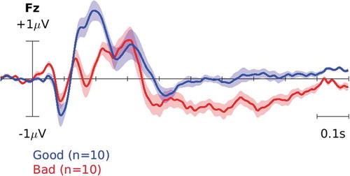
Figure 5. ERP in dataset II. The blue curve corresponds to the brain response to ‘good’ cursor movements, i.e. toward the target. The red curve, on the other hand, corresponds to the brain response to ‘bad’ movements, i.e. away from the target.
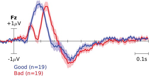
Table 1. Dataset I: G/B classification accuracy using spatial and temporal features separately. Each table entry is the average classification accuracy (first number) together with the standard error of the mean (second number) over 10 instances of train-test for each participant. Riemannian methods outperform their counterparts and this difference is significant across participants (paired-sample t-test, ).
Table 2. Dataset II: G/B classification accuracy using spatial and temporal features separately. Each table entry is the average classification accuracy (first number) together with the standard error of the mean (second number) over 10 instances of train-test for each participant. DRM-T outperforms its counterpart and this difference is significant across participants (paired-sample t-test, ). However, the difference between CSP and DRM-S is not statistically significant.
Table 3. Dataset I: G/B classification accuracy comparing the proposed spatio-temporal methods and WM. Each table entry is the average classification accuracy (first number) together with the standard error of the mean (second number) over 10 instances of train-test for each participant. Significantly improved results across participants are represented in bold fonts (paired-sample t-test, , which stays significant at the 0.05 threshold with Bonferroni correction for the number of tests, i.e. 4).
Table 4. Dataset II: G/B classification accuracy comparing the proposed spatio-temporal methods and WM. Each table entry is the average classification accuracy (first number) together with the standard error of the mean (second number) over 10 instances of train-test for each participant. Significantly improved results across participants are represented in bold fonts (paired-sample t-test, , which stays significant at the 0.05 threshold with Bonferroni correction for the number of tests, i.e. 4).
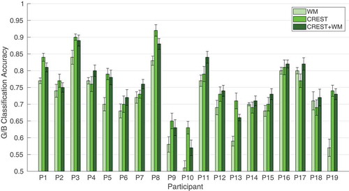
Figure 6. WM, CREST and CREST+WM in dataset I. The bars and error bars represent the average classification accuracy and the standard error of the mean, respectively, i.e. first and second entries in columns 2, 5 and 6.
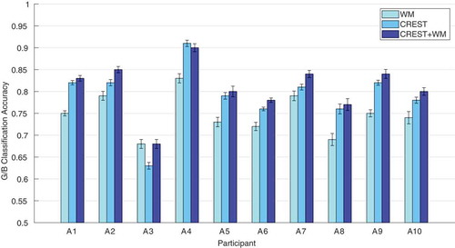
Figure 7. WM, CREST and CREST+WM in dataset II. The bars and error bars represent the average classification accuracy and the standard error of the mean, respectively, i.e. the first and second entries in columns 2, 5 and 6.