Feasibility of decoding visual information from EEG

Figures & data

Figure 1. Classic pipeline for decoding visual information. First the neural signal is measured whilst the individual performs a visual imagery or perception task. This neural signal is then decoded. The output contents include an example of pictorial reconstruction (a), semantic classification (b), and identification of low level visual information such as shape (c) and colour (d).

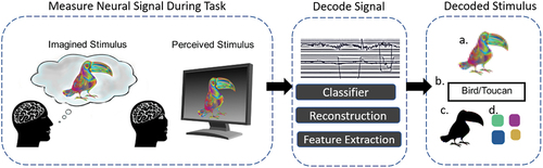
Figure 2. This demonstrates the relative speed taken to process similar information content in either a. visual or b. auditory modalities. Object recognition, such as this glacier scene, can be detected as early as 100ms from visual perception, figure taken and adapted from Lowe et al. [29]. How long does it take to say the sentence out loud in B?

Figure 3. This demonstrates key regions related to visual processing, such as V1–3 and the lateral geniculate nucleus.This image is adapted and taken from BodyParts3D, © the Database center for Life Science licensed under CC attribution-share alike 2.1 Japan.

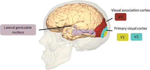
Table 1. Key words used to identify papers included in the following literature review for each target.

Target	Key word variations
BCI	BCI; brain computer interface; brain-computer interface; BMI; brain-machine interace; brain machine interface
EEG	eeg; electroencephalography; electroencephalogram
visual imagery	visual imagery; mental imagery; visual imagination; mind’s eye; imagined picture(s); picture imagery; mental picture(s)
visual perception	visual perception; seeing; vision; looking;
shape	shape(s); orientation(s); location(s); position(s); geometric; size(s); spatial
colour	colour(s); colour(s); RGB; hue(s); colourimetry
texture	texture(s);
naturalistic	naturalistic; natural; complex; scene(s); face(s); place(s); object(s); digit(s); letter(s); character(s)

Table 4. Simple visual features EEG datasets.

Author	Task	Stimuli	Device	Channels	Sampling Rate	Duration
Spatial Information Decoding
Llorella et al. [44]	Imagination	7 geometric shapes and then 2 geometric shapes	g.Nautilus g.tec	8 channels - P3, P4, PO3, POz, PO4, PO7, PO8 and Oz	Recorded at 250 Hz	Imagination duration 5000 ms
Qiao et al. [45]	Perception	8 spatial patterns	Neuroscan	64 channels	Recorded at 1000 Hz	Perception duration of 4000 ms
Esfahani and Sundararajan [46],	Perception and Imagination	5 shapes	emotiv neuroheadset	14 channels - AF3, F7, F3, FC5, T7, P7, O1, O2, P8, T8, FC6, F4, F8, AF4	Recorded at 2048 Hz, then down sampled to 128 Hz	Perception duration of 2000 ms and imagination duration of 5000 ms
Gurariy et al. [47]	Perception	Shape vs Tool Images	HydroCel Geodesic Sensor Net	256 channels	Recorded at 1000 Hz	Perception duration of 300 ms
Texture Decoding
Portilla and Simoncelli [48],	Perception	166 natural texture images	Brainvision	19 channels - Fp1, Fp2, F3, F4, C3, C4, P3, P4, O1, O2, F7, F8, T7, T8, P7, P8, Fz, Cz, and Pz	Recorded at 1000 Hz	Perception 500 ms
Colour Decoding
Yu and Sim [49]	Passive perception, and imagination	red, green, blue, white, and yellow LED lights	Emotiv Epoc	14 channels - AF3, F7, F3, FC5, T7, P7, O1, O2, P8, T8, FC6, F4, F8, and AF4	128 Hz	Perception 7000 ms and imagination 7000 ms
Hajonides et al. [50]	Perceive then recall orientation and colour of two simultaneous gabor patches	Gabor patches, 48 colour variations, 48 orientation variations. 900 trials per participant	EasyCap	61 channels	1000 Hz	Perception 300 ms
Rasheed [51]	Passive perception, and imagination	red, green, blue and grey squares; 60 trials for each colour per participant	G.tec’s g.MOBIlab+ portable device	4 channels - P3, P4, O1 and O2	256 Hz	Perception 3000 ms; Imagination 3000 ms

Figure 4. Types of stimuli used in the three mentioned colour decoding studies; a) shows examples of coloured Gabor patch stimuli, b) depicts the coloured square on a curved projector in Rasheed [51] and c) shows the Arduino with led lights used in Yu and Sim [49]. B and C images are adapted from their respective papers.

Table 2. Decoding performance metrics for colour, including details on the classifier employed, feature extraction methods, spatial areas selected, chosen time windows, and the calculation of information transfer rate (ITR).

Study	N -Class	Classifier	Features	Spatial selection	Time (sec)	Accuracy	ITR (bpm)
Hajonides (Perception)	2	LDA	PCA	posterior occipital	0.35	$\sim$	$\sim$
Wu (Perception)	2	SVM	Cleaned EEG	primary visual cortex	1	>70%	7.12
Yu (Imagination)	5	ANN	alpha, beta waves	T7, F4, AF4	7	61.5	0.3
Torres-Garcia (Perception)	3	RF	statistical features	P1, P2, O1, O2	3	38	1.2
Torres-Garcia (Imagination)	3	SVM	statistical features	P1, P2, O1, O2	3	36	0.9

Figure 5. In this figure depicted are: a. The geometric shapes used in [46] b. seven geometric shapes from [44].

Table 3. Decoding performance metrics for spatial features, including details on the classifier employed, feature extraction methods, spatial areas selected, chosen time windows, and the calculation of information transfer rate (ITR).

Study	Class (N)	Classifier	Features	Spatial selection	Time window (sec)	Accuracy	ITR (bpm)
Llorella et al. (imagination)	2	CNN	EEG	posterior occipital	5	70%	5.8
Esfahani et al. (imagination)	5	LDA	Hilbert-Huang Transform	global	5	44.6%	2.6
Qiao et al (perception)	8	CNN-LSTM	$\sim$	posterior occipital	4	70	9.7
Gurariy et al. (Perception)	2	MVPA	EEG	ventral dorsal	0.055 onwards	$\sim$	$\sim$

Figure 6. a) shows reconstructions using MVAE wakita et al. [70] and b) are reconstructions from Orima and Motoyoshi [71] using the figure is adapted from Orima and Motoyoshi [71]; wakita et al. [70].

Table 5. Decoding performance metrics for complex stimuli, including details on the classifier employed, feature extraction methods, spatial areas selected, chosen time windows, and the calculation of information transfer rate (ITR).

Study	N -Class	Classifier	Features	Spatial selection	Time (sec)	Accuracy	ITR (bpm)
Kumar et al. (imagination)	3	RF	Statistical features	global	10	85.2%	5
Tirupattur et al (imagination)	10	CNN LSTM	EEG	global	10	$\sim$72%	2.7
Nemrodov et al. (perception)	2	SVM	EEG	occipito-temporal	0.05 to 650	71%	13.1
Shatek et al. (perception)	2	Linear Discriminant	EEG	global	0.12	$\sim$58%	9.27
Kosmyna et al. (perception)	2	Logistic Regression	SpecCSP	global	2	60%	1.1
Kosmyna et al. (imagination)	2	Logistic Regression	SpecCSP	global	2	52%	0.03

Table 6. Datasets for naturalistic/complex stimuli relaying stimuli details, acquisition device, sampling rate and duration of the imagination or perception task.

Author	Task	Stimuli	Device	Channels	Sampling Rate	Duration
Kumar et al. [72]	Perceive and imagine	colour digits (0–9); non-text objects; letters	Emotiv EPOC+	14 channels	128Hz (downsampled from 2048 Hz)	Perception: 10000ms, Imagination: 1,000ms
Nemrodov et al. [73]	Perceive, go trials in a go/no-go gender recognition task	Unfamiliar male faces, 54 happy and 54 neutral expressions	Biosemi ActiveTwo EEG recording system	64 channels	512 Hz	Perception: 300 ms
Shatek et al. [74]	Perceive four images, then imagine one of these, then select which one chosen for imagination	Variations of Sydney Harbour Bridge, and Santa-Claus (40 trials per class, 80 in total)	Brain Products ActiCAP	64 channels	1000 Hz	Perception: 1,500 ms, Imagination: 3,000ms
Kosmyna et al. [75]	Visual observation followed by visual imagination	Two simplified pictures on black background 1) daisy, 2) hammer	2 g.tec USBAmp amplifiers	36 channels		Perception: 4,000ms, Imagination: 4,000ms
Spampinato et al. [76]	Passively perceive images	Various objects scuh as dog, cat, butterfly, sorrel, capuchin, elephant, panda, fish, airliner, broom, canoe, phone, mug, convertible, computer	Brainvision DAQs and amplifiers with actiCAP	128 channels	1000 Hz	Perception: 500ms
Rashkov et al. [77]	Passively perceive video clips of different objects	Abstract geometric shapes, waterfalls, human faces, goldberg mechanisms, extreme sports	NVX-136 amplifier developed by Medical Computer Systems Ltd. (Moscow, Zelenograd)	128 channels	500 Hz	Single clip was 6,000 to 10000ms

Figure 7. Examples of the unfamiliar male faces used. The top row are the original displayed faces, the bottom row are their respective reconstructions. Adapted from Nemrodov et al. [73].

Figure 8. Showing the types of binary stimuli used. In a) classification of an imagined/perceived hammer vs. A flower adapted from Kosmyna et al. [75], b) classification of Sydney Harbour bridge vs. Santa Claus adapted from Shatek et al. [74].

Figure 9. Examples of reconstruction results from Zheng et al. [84].

Figure 10. Illustrates that at the time of this review, at least eight further visual decoding studies have been carried out which use Spampinato et al. [76]’s foundational dataset.

Table 7. This table compares the relative cost, spatial and temporal resolution, portability, and invasiveness of the neuroimaging modalities discussed in this current section on EEG hardware.

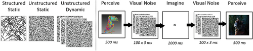
Figure 11. The left side depicts the difference between unstructured, structured and dynamic visual noise. For unstructured dynamic, black and white dots are selected at random with multiple iterations. This example shows three random dot variations shown consecutively. The right hand side depicts how visual noise can be injected into the experiment pipeline, before and after each perception and imagery task.

Lowe MX, Rajsic J, Ferber S, et al. Discriminating scene categories from brain activity within 100 milliseconds. Cortex. 2018;106:275–287. doi: 10.1016/j.cortex.2018.06.006

 PubMed Web of Science ®Google Scholar

Llorella FR, Iáñez E, Azorn JM, et al. Classification of imagined geometric shapes using eeg signals and convolutional neural networks. Neurosci Inform. 2021;1(4):100029. doi: 10.1016/j.neuri.2021.100029

 Google Scholar

Qiao J, Tang J, Yang J, et al. Basic graphic shape decoding for eeg-based brain-computer interfaces. In 2021 43rd Annual International Conference of the IEEE Engineering in Medicine & Biology Society (EMBC), IEEE; 2021. p. 812–815.

 Google Scholar

Esfahani ET, Sundararajan V. Classification of primitive shapes using brain–computer interfaces. Comput Aided Des. 2012;44(10):1011–1019. doi: 10.1016/j.cad.2011.04.008

 Web of Science ®Google Scholar

Gurariy G, Mruczek RE, Snow JC, et al. Using high-density electroencephalography to explore spatiotemporal representations of object categories in visual cortex. J Cognitive Neurosci. 2022;34(6):967–987. doi: 10.1162/jocn_a_01845

 PubMed Web of Science ®Google Scholar

Portilla J, Simoncelli EP. A parametric texture model based on joint statistics of complex wavelet coefficients. Int J Comput Vis. 2000;40(1):49–70. doi: 10.1023/A:1026553619983

 Web of Science ®Google Scholar

Yu J-H, Sim K-B. Classification of color imagination using Emotiv EPOC and event-related potential in electroencephalogram. Optik. 2016;127(20):9711–9718. doi: 10.1016/j.ijleo.2016.07.074

 Web of Science ®Google Scholar

Hajonides J, van Ede F, Nobre K, et al. Parametric decoding of visual colour from contralateral scalp electroencephalography. J Vis. 2020;20(11):1139–1139. doi: 10.1167/jov.20.11.1139

 Google Scholar

Rasheed S. Recognition of primary colours in electroencephalograph signals using support vector machines. Università degli Studi di Milano. 2011.

 Google Scholar

Wakita S, Orima T, Motoyoshi I. Photorealistic reconstruction of visual texture from eeg signals. Front Comput Neurosci. 2021;15:15. doi: 10.3389/fncom.2021.754587

 Web of Science ®Google Scholar

Orima T, Motoyoshi I. Analysis and synthesis of natural texture perception from visual evoked potentials. Front Neurosci. 2021;15:876. doi: 10.3389/fnins.2021.698940

 Web of Science ®Google Scholar

Kumar P, Saini R, Roy PP, et al. Envisioned speech recognition using EEG sensors. Pers Ubiquitous Comput. 2018;22(1):185–199.

 Web of Science ®Google Scholar

Nemrodov D, Niemeier M, Patel A, et al. The neural dynamics of facial identity processing: insights from EEG-based pattern analysis and image reconstruction. eNeuro. 2018;5(1):ENEURO.0358–17.2018.

 PubMed Web of Science ®Google Scholar

Shatek SM, Grootswagers T, Robinson AK, et al. Decoding images in the mind’s eye: the temporal dynamics of visual imagery. Vision. 2019;3(4):53. doi: 10.3390/vision3040053

 Google Scholar

Kosmyna N, Lindgren JT, Lécuyer A. Attending to visual stimuli versus performing visual imagery as a control strategy for EEG-based brain-computer interfaces. Sci Rep. 2018;8(1):1–14. doi: 10.1038/s41598-018-31472-9

 PubMedGoogle Scholar

Spampinato C, Palazzo S, Kavasidis I, et al. Deep learning human mind for automated visual classification. In Proceedings of the IEEE conference on computer vision and pattern recognition; Honolulu, HI, USA; 2017. p. 6809–6817.

 Google Scholar

Rashkov G, Bobe A, Fastovets D, et al. Natural image reconstruction from brain waves: a novel visual bci system with native feedback. bioRxiv. 2019;787101.

 Google Scholar

Zheng X, Chen W, Li M, et al. Decoding human brain activity with deep learning. Biomedical Signal Processing And Control. 2020a;56:101730. doi: 10.1016/j.bspc.2019.101730

 Web of Science ®Google Scholar