How do linguistic illusions arise? Rational inference and good-enough processing as competing latent processes within individuals

Figures & data

Table 1. Constructions used in the experimental study.

Inversion: Order of direct and indirect object is swapped (e.g. Gibson et al., 2013)

The mother gave the candle the daughter.

Agreement attraction: Verb agrees with intervening noun phrase instead of subject noun phrase (e.g. Bock et al., 2001)

The waitress who sat the girls unsurprisingly were unhappy about all the noise.

Depth charge: Incongruous degree phrase “saved” by negation (e.g. Wason & Reich, 1979)

In Maria's class, no test is too difficult to fail.

Comparative illusion: Number of individuals compared to number of events (e.g. Wellwood et al., 2018)

More engineers relocated to San Francisco than our accountant did.

Missing VP illusion: Three clauses with three subjects but only two verbs (e.g. Gibson & Thomas, 1999)

The manuscript that the student who the catalog had confused was missing a page.

NPI illusion: Negative polarity item (NPI) ever licensed by embedded negation (e.g. Drenhaus et al., 2005)

The authors that no critics recommended have ever received acknowledgment for a novel.

Figure 1. Judgment options as during the experiment.

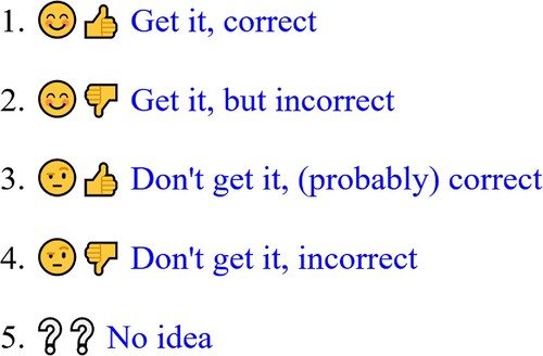
Figure 2. Response proportions across constructions and conditions.

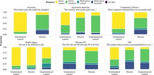
Figure 3. Judgment times (reading time + response selection time) across constructions, conditions, and response types. Note that the y-axis is log-scaled.

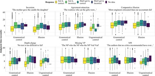
Table 2. Factor loadings from the principal components analysis of the questionnaire data.

	Factor 1	Factor 2
	(pedantry)	(charity)
had fun	0.62	0.58
bothered by incorrect grammar	0.66	−0.46
assume that people make sense	−0.16	0.82
attentive reading	0.84	0.09

Figure 4. Contributions of component processes to the finishing times of the three accumulators in a hypothetical experimental trial.

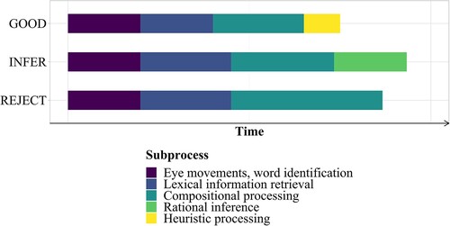
Figure 5. Posterior predictive distributions of finishing times (250 samples) of the three accumulators across constructions and conditions. Faster finishing times correspond to a higher expected number of responses of the respective type. Finishing times more than ± 2.5 SD away from the log mean have been removed. Reference line added at 8 seconds. Note that the x-axis is log-scaled.

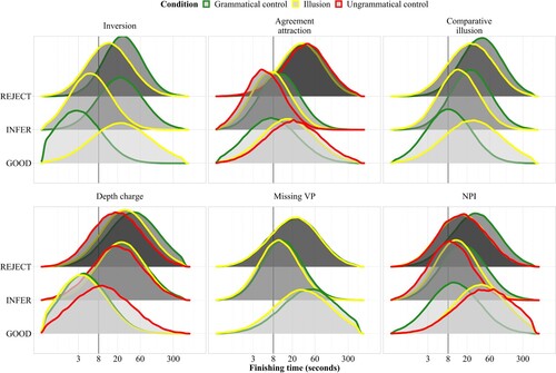
Figure 6. 95% highest density intervals of slope parameters across all constructions on the log ms scale. Across all constructions, the slope is the difference between the illusion condition and the indicated control condition(s). Positive estimates correspond to a slowdown of the accumulator, that is, fewer responses of the associated category in the illusion condition. Reference line added at $0\log$ ms.

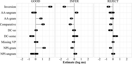
Figure 7. Mean ± 2 SD of predicted accumulator finishing times (250 samples) for the illusion condition across constructions. Faster finishing times correspond to a higher expected number of responses of the respective type. Finishing times more than ±2.5 SD away from the log mean have been removed. Reference line added at 8 seconds. Note that the x-axis is log-scaled.

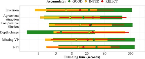
Figure 8. Predicted (colored) versus observed (gray) response proportions across constructions and conditions. Proportions were computed by participant. The visible stratification is due to between-participant variability, which is accurately captured by the model.

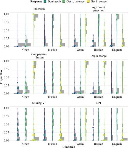
Figure 9. Predicted (histograms) versus observed (eye plots) judgment time distributions across constructions, conditions, and responses.

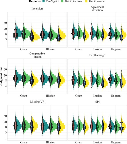
Figure 10. Histogram of subject-level random-effects correlations across all constructions by accumulator pair, weighted by probability of direction.

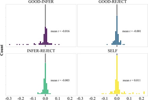
Figure 11. Correlation estimates of subject-level random effects and associated 95% highest density intervals. Only correlations with probability of direction >0.95 for slope parameters (differences between conditions) are shown.

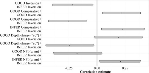
Figure 12. Posterior predictive distributions of finishing times (250 samples) of the three accumulators across constructions and conditions, by pedantry score. Interactions with probability of direction >0.95 are highlighted in blue.

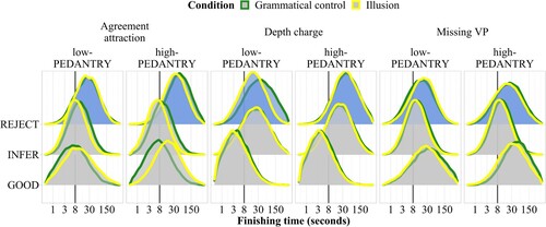
Figure 13. Posterior predictive distributions of finishing times (250 samples) of the three accumulators across constructions and conditions, by charity score. Interactions with probability of direction >0.95 are highlighted in blue.

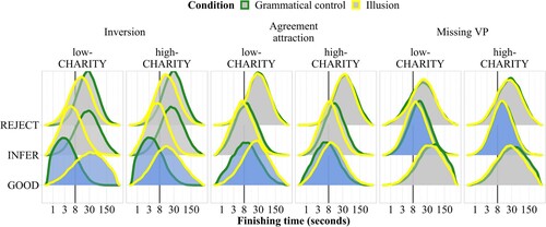
Figure 14. Posterior predictive distributions of finishing times (250 samples) of the three accumulators across constructions and conditions, by logic score. Interactions with probability of direction >0.95 are highlighted in blue.

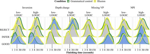
Figure 15. Posterior predictive distributions of finishing times (250 samples) of the three accumulators across constructions and conditions, by conflict score. Interactions with probability of direction >0.95 are highlighted in blue.

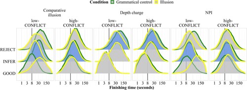
Figure 16. Estimated differences in log pointwise predictive density between the full model and alternative models. A positive difference means that the alternative model has a better predictive fit than the full model. Error bars show 95% confidence intervals. Note that the y-axis is square-root-scaled.

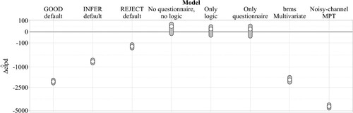
Figure 17. Difference in log pointwise predictive density between the full race model and the noisy-channel MPT model by condition, response, and judgment time.

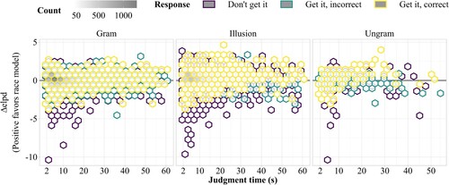
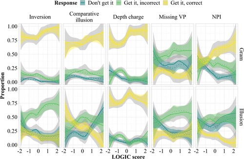
Figure 18. LOESS curves of response proportions by logic score, construction, and condition. Solid lines are based on the experimental data; dotted lines are based on model predictions.

Gibson, E., Bergen, L., & Piantadosi, S. T. (2013). Rational integration of noisy evidence and prior semantic expectations in sentence interpretation. Proceedings of the National Academy of Sciences, 110(20), 8051–8056. https://doi.org/10.1073/pnas.1216438110

 PubMed Web of Science ®Google Scholar

Bock, K., Eberhard, K. M., Cutting, J. C., Meyer, A. S., & Schriefers, H. (2001). Some attractions of verb agreement. Cognitive Psychology, 43(2), 83–128. https://doi.org/10.1006/cogp.2001.0753

 PubMed Web of Science ®Google Scholar

Wason, P. C., & Reich, S. S. (1979). A verbal illusion. The Quarterly Journal of Experimental Psychology, 31(4), 591–597. https://doi.org/10.1080/14640747908400750

 PubMed Web of Science ®Google Scholar

Wellwood, A., Pancheva, R., Hacquard, V., & Phillips, C. (2018). The anatomy of a comparative illusion. Journal of Semantics, 35(3), 543–583. https://doi.org/10.1093/jos/ffy014

 Web of Science ®Google Scholar

Gibson, E., & Thomas, J. (1999). Memory limitations and structural forgetting: The perception of complex ungrammatical sentences as grammatical. Language and Cognitive Processes, 14(3), 225–248. https://doi.org/10.1080/016909699386293

 Web of Science ®Google Scholar

Drenhaus, H., Saddy, D., & Frisch, S. (2005). Processing negative polarity items: When negation comes through the backdoor. In S. Kepser & M. Reis (Eds.), Linguistic evidence: Empirical, theoretical, and computational perspectives (pp. 145–165). Mouton de Gruyter.

 Google Scholar

Data availability

The experimental data, as well as all analysis and modelling code, are available at https://osf.io/5gnk7.

Data availability statement

All experimental materials, data and analysis code are available at https://osf.io/5gnk7.