1,071
Views
2
CrossRef citations to date
0
Altmetric
Research Article

Picard’s iterative method for nonlinear multicomponent transport equations

ORCID Icon | (Reviewing Editor)
Article: 1158510 | Received 27 Oct 2015, Accepted 20 Feb 2016, Published online: 30 Mar 2016

Figures & data

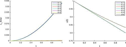
Figure 1. The two-level Picard’s method compared with the analytical solution.

Figure 1. The two-level Picard’s method compared with the analytical solution.

Table 1. Comparative results of the two-level method with k iterative steps and the analytical solution for Δt=10-2 and T=1.0

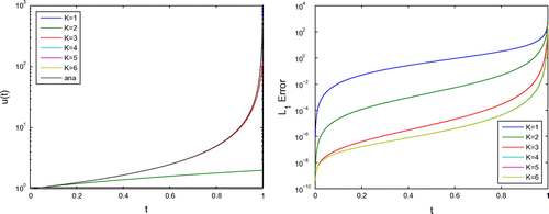
Figure 2. The three-level Picard’s method compared with the analytical solution.

Figure 2. The three-level Picard’s method compared with the analytical solution.

Table 2. Comparative results of the three-level method with k iterative steps and the analytical solution for Δt=10-2 and T=1.0

Figure 3. The two-level Picard’s method compared with the analytical solution.

Figure 3. The two-level Picard’s method compared with the analytical solution.

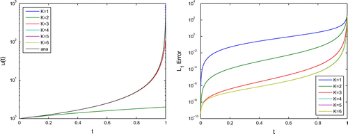
Figure 4. The three-level Picard’s method compared with the analytical solution.

Figure 4. The three-level Picard’s method compared with the analytical solution.

Figure 5. The three-level Picard’s method compared with the analytical solution (left side: solutions, right side: errors between analytical and numerical methods).
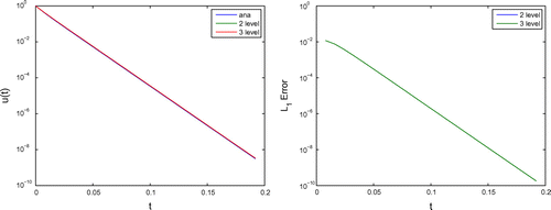
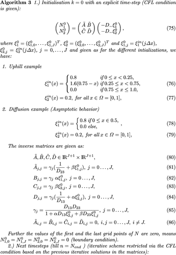
Figure 5. The three-level Picard’s method compared with the analytical solution (left side: solutions, right side: errors between analytical and numerical methods).
Figure 6. The numerical error of general Picard’s fix-point method and a reference solution (fourth-order RK-method with fine time steps).
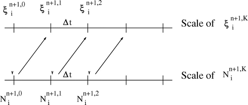
Figure 6. The numerical error of general Picard’s fix-point method and a reference solution (fourth-order RK-method with fine time steps).

Figure 7. The numerical solution of the three- and four-level Picard’s fix-point methods with different iterative steps.
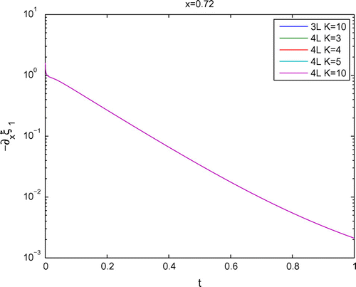
Figure 7. The numerical solution of the three- and four-level Picard’s fix-point methods with different iterative steps.
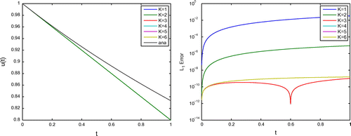
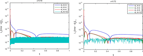
Figure 8. The figures present the numerical L1-error between the four-level Picard’s fix-point scheme and the reference solution for different iterative steps (left figure: high resolution of the error, right figure: low resolution based on averaging the high oscillating errors).

Figure 8. The figures present the numerical L1-error between the four-level Picard’s fix-point scheme and the reference solution for different iterative steps (left figure: high resolution of the error, right figure: low resolution based on averaging the high oscillating errors).

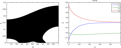
Figure 9. The figures present the numerical solutions of the uphill experiment (left side) and the concentrations at spatial point x=0.72 with a four-level Picard’s fix-point scheme computed (right side).

Figure 9. The figures present the numerical solutions of the uphill experiment (left side) and the concentrations at spatial point x=0.72 with a four-level Picard’s fix-point scheme computed (right side).