3,204
Views
15
CrossRef citations to date
0
Altmetric
Research Article

A novel approach for numeric study of 2D biological population model

| (Reviewing Editor)
Article: 1261527 | Received 08 Jul 2016, Accepted 10 Nov 2016, Published online: 02 Dec 2016

Figures & data

Table 1. Comparison of numerical solution of Example 1 at x=0.5,y=0.5

Table 2. The errors in Example 1 at different time levels t0.5

Table 3. The errors in Example 1 for large time levels 5t20 with hx=hy=1/12

Table 4. Rate of convergence (ROC) of Example 1

Table 5. Errors in BPM given in Example 2 at 0t1.0 for different time steps and hx=hy=0.1

Table 6. Errors in BPM given in Example 2 at 0t1.0 with t=0.0001

Table 7. The errors in Example 2 for large time levels 5t20 with hx=hy=1/12

Table 8. Rate of convergence of Example 2

Table 9. Comparison of numerical solution of Example 3 at x=0.5,y=0.5

Table 10. The errors in Example 3 for large time levels 2t10 with hx=hy=1/12

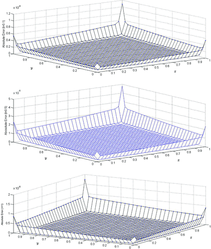
Figure 1. The absolute errors BPM in Example 1 at different time levels t1 with parameters hx=hy=0.04,t=0.0001.

Figure 1. The absolute errors BPM in Example 1 at different time levels t≤1 with parameters hx=hy=0.04,▵t=0.0001.

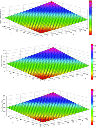
Figure 2. The approximate solution of BPM in Example 1 at different time levels t1 with parameters hx=hy=0.04,t=0.0001.

Figure 2. The approximate solution of BPM in Example 1 at different time levels t≤1 with parameters hx=hy=0.04,▵t=0.0001.

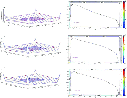
Figure 3. Contour and surface plot of absolute errors of ρ(x,t) given in Example 2 for t=0.1,0.5,1 with parameters hx=hy=0.05,t=0.0001.

Figure 3. Contour and surface plot of absolute errors of ρ(x,t) given in Example 2 for t=0.1,0.5,1 with parameters hx=hy=0.05,▵t=0.0001.

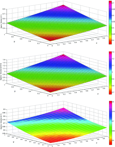
Figure 4. The behavior of ρ(x,t) in Example 2 for t=0.1,0.5,1 with parameters hx=hy=0.05,t=0.0001.

Figure 4. The behavior of ρ(x,t) in Example 2 for t=0.1,0.5,1 with parameters hx=hy=0.05,▵t=0.0001.

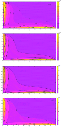
Figure 5. Contour plot of absolute errors of ρ(x,t) in Example 3 for t=0.1,0.2,0.3,0.5 with parameters hx=hy=0.05,t=0.0001.

Figure 5. Contour plot of absolute errors of ρ(x,t) in Example 3 for t=0.1,0.2,0.3,0.5 with parameters hx=hy=0.05,▵t=0.0001.

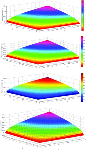
Figure 6. Surface behavior of BPM as given in Example 3 for t=0:1;0:2;0:3;0:5 with parameters hx=hy=0:05;t=0:0001.

Figure 6. Surface behavior of BPM as given in Example 3 for t=0:1;0:2;0:3;0:5 with parameters hx=hy=0:05;▵t=0:0001.