1,734
Views
2
CrossRef citations to date
0
Altmetric
Research Article

A comparative numerical study of turbulence models for the simulation of fire incidents: Application in ventilated tunnel fires

, , & | (Reviewing Editor)
Article: 1000509 | Received 10 Jul 2014, Accepted 16 Dec 2014, Published online: 09 Jan 2015

Figures & data

Figure 1. Sketch of the tunnel and heat source.

Figure 1. Sketch of the tunnel and heat source.

Table 1. Coefficients of Equation 1 and constants values

Table 2. Cases data and calculated results

Figure 2. Numerical mesh used for the standard kε with wall functions simulations.

Notes: Section y = 2.7 m near the vicinity of the heat source (top figure). Cross-section x = 60 m (bottom figure).
Figure 2. Numerical mesh used for the standard k–ε with wall functions simulations.
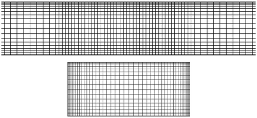
Figure 3. Numerical mesh used for the low-Re kω SST simulations.

Notes: Section y = 2.7 m near the vicinity of the heat source (top figure). Cross-section x = 60 m (bottom figure).
Figure 3. Numerical mesh used for the low-Re k–ω SST simulations.
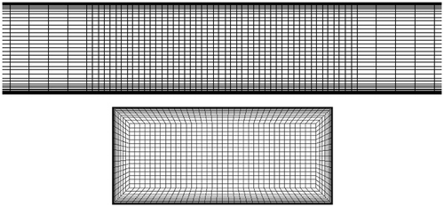
Figure 4. Temperature isolines through time for case 1.
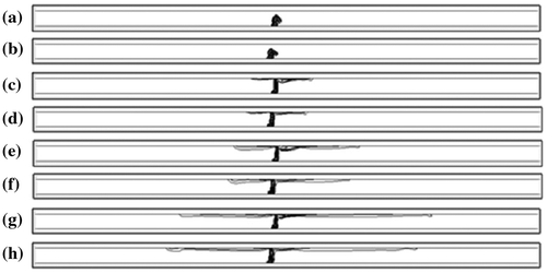
Notes: (a) Standard kε at 0.5 s; (b) Low-Re kω SST at 0.5 s; (c) Standard kε at 2 s; (d) Low-Re kω SST at 2 s; (e) Standard kε at 5 s; (f) Low-Re kω SST at 5 s; (g) Standard kε at 10 s; and (h) Low-Re kω SST at 10 s.
Figure 4. Temperature isolines through time for case 1.

Figure 5. Temperature isolines through time for case 2.
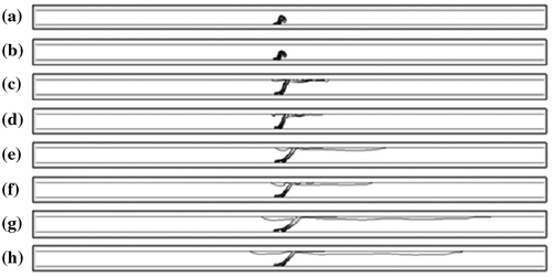
Notes: (a) Standard kε at 0.5 s; (b) Low-Re kω SST at 0.5 s; (c) Standard kε at 2 s; (d) Low-Re kω SST at 2 s; (e) Standard kε at 5 s; (f) Low-Re kω SST at 5 s; (g) Standard kε at 10 s; and (h) Low-Re kω SST at 10 s.
Figure 5. Temperature isolines through time for case 2.

Figure 6. Velocity vectors at characteristic sections and moments for case 1 predicted by the standard kε model (left column) and the low-Re kω SST model (right column).

Notes: Section y = 2.7 m near the heat source at 0.5 s (top row), cross-section x = 60 m at 1 s (middle row), and cross-section x = 60 m at 5 s (bottom row).
Figure 6. Velocity vectors at characteristic sections and moments for case 1 predicted by the standard k–ε model (left column) and the low-Re k–ω SST model (right column).
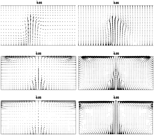
Figure 7. Velocity vectors at characteristic sections and moments for case 2 predicted by the standard kε model (left column) and the low-Re kω SST model (right column).

Notes: Section y = 2.7 m near the heat source at 0.5 s (top row), cross-section x = 62 m at 1 s (middle row) and cross-section x = 62 m at 5 s (bottom row).
Figure 7. Velocity vectors at characteristic sections and moments for case 2 predicted by the standard k–ε model (left column) and the low-Re k–ω SST model (right column).
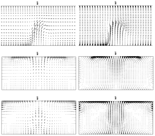
Figure 8. Case 2, 20 s after fire breaking.
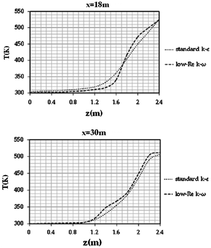
Notes: Vertical temperature profiles at a distance of 18 m (top figure) and 30 m (bottom figure) downstream from the heat source.
Figure 8. Case 2, 20 s after fire breaking.

Figure 9. Convergence curve.
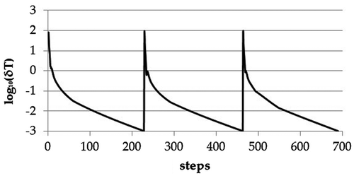
Notes: Temperature corrections in pseudo-time for three physical time steps with starting point t = 2 s.
Figure 9. Convergence curve.

Figure 10. Flame shape comparison for case 1.
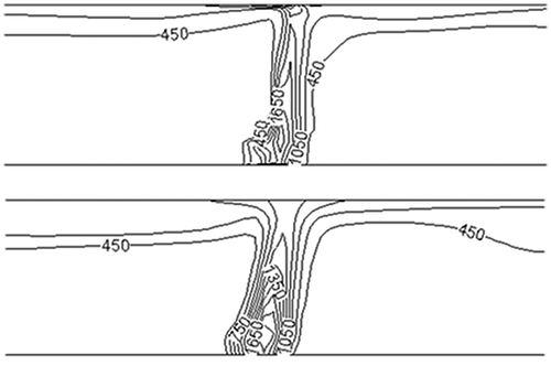
Notes: Present solver with the kω model (top figure), Ansys Fluent with the kε model (bottom figure).
Figure 10. Flame shape comparison for case 1.

Figure 11. Flame shape comparison for case 2.
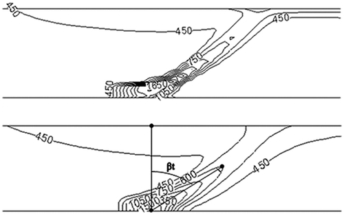
Notes: Present solver with the kε model (top figure), Ansys Fluent with kε model (bottom figure). Definition of flame angle.
Figure 11. Flame shape comparison for case 2.

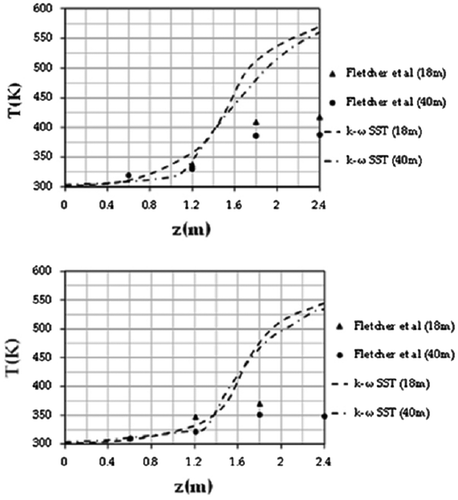
Figure 12. Comparison of temperature profiles along height when steady state was reached.

Notes: Case 1 (top figure), and case 2 (bottom figure).
Figure 12. Comparison of temperature profiles along height when steady state was reached.

Figure 13. Velocity vectors at section y = 2.7 m and stagnation point (red circle).

Figure 13. Velocity vectors at section y = 2.7 m and stagnation point (red circle).