Bi-objective evolutionary optimization of level of service in urban transportation based on traffic density

Figures & data

Figure 15. PM emission difference between A8b and A8a.

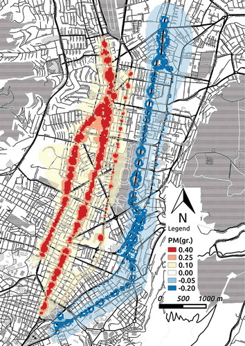
Figure 1. Method.

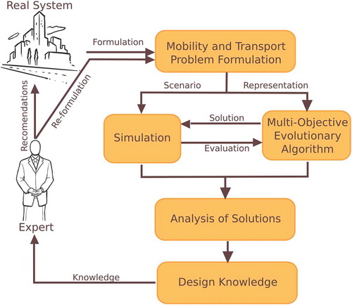
Figure 2. DMQ BRT scenario.

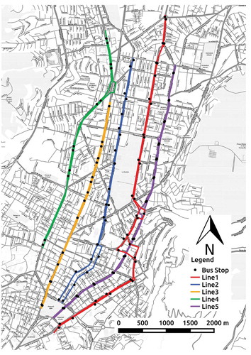
Figure 3. Simulation and EA integration.

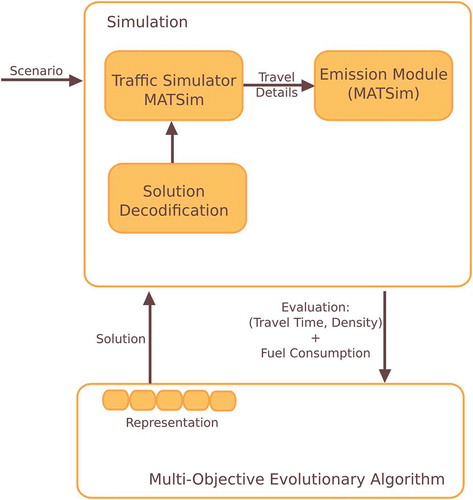
Figure 4. Solution representation.

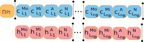
Table 1. Automobile distribution (fuel = gasoline and weight ≤ 2 Tons)

Year-Category	%	Year-Category	%
2000–2002|Euro2	24.40	2008–2010|Euro5	13.70
2002–2004|Euro3	7.80	2010–2012|Euro6	23.80
2004–2006|Euro4	12.20	2012–2014|Euro6	5.20
2006–2008|Euro4	13.00

Figure 5. Hyper volumeover generations.

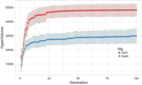
Figure 6. Hyper volumeover generations of one run.

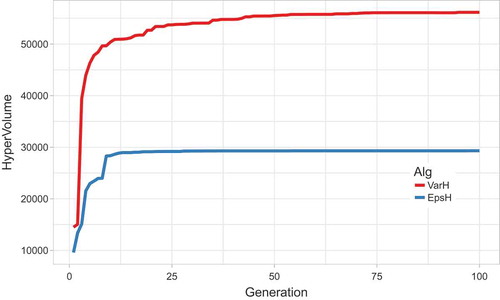
Figure 7. Pareto optimal set of one run.

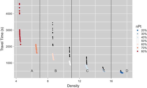
Figure 8. Travel time and density, colored by fraction of public transport users $n_{Pt}$. Black dots show POS founded by the original algorithm.

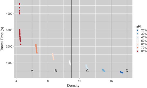
Table 2. Two set coverage index (C)

	Mean	SD
C(A$\epsilon$S$\epsilon$H,A$\epsilon$S$v$H)	0.24	0.18
C(A$\epsilon$S$v$H,A$\epsilon$S$\epsilon$H)	0.50	0.31

Table 3. Objective correlation matrix

	tt	dens	fc
tt	—	−0.91	−0.92
dens	−0.91	—	0.99
fc	−0.92	0.99	—

Table 4. Levels of service for basic freeways segments

Levels of	Density
service	(pc/km/ln)
A	0–7
B	7–11
C	11–16
D	16–22
E	22–28
F	> 28

Figure 9. Fuel consumption and travel time, colored by level of service.

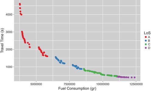
Figure 10. Fuel consumption and density, colored by fraction of public transport users ${\mathit{n}}_{\mathit{P}\mathit{t}}$.

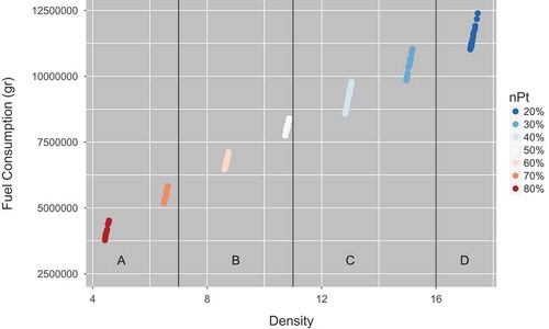
Figure 11. Trade-off TT and PM by ${\mathit{n}}_{\mathit{P}\mathit{t}}$.

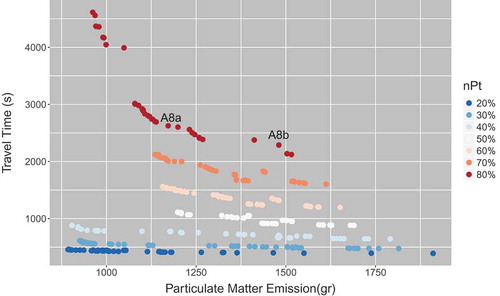
Figure 12. Number of public transportation trips by ${\mathit{n}}_{\mathit{P}\mathit{t}}$.

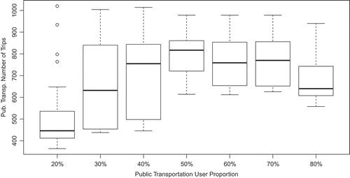
Figure 13. Public transportation PM emission by ${\mathit{n}}_{\mathit{P}\mathit{t}}$.

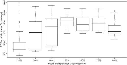
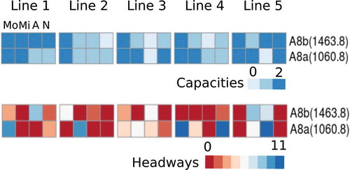
Figure 14. Configuration of bus capacities (top) and headways (bottom) of solutions A8b and A8a. Schedules: Mo, Mi, A, N (morning, midday, afternoon, night). Capacities: 0, 1, 2 (small, medium, large). Headways: 0,…, 11 (5 min, …, 60 min).