On the prediction capabilities of two SGS models for large-eddy simulations of turbulent incompressible wall-bounded flows in OpenFOAM

Figures & data

Figure 1. Channel geometry used for each simulation in this work. Boundary conditions: abcd: Cyclic; efgh: Cyclic; abfe: Cyclic; dcgh: Cyclic; bcgf: Wall; adhe: Wall

Table 1. Numerical schemes employed for all simulations performed in this work

Term	Numerical scheme	Accuracy
Time derivative	Crank Nicholson	2nd order
Gradient	Fourth	4th order
Divergence	Gauss cubic	3rd order
Laplacian	Gauss cubic corrected	3rd order
Surface normal gradient	Fourth	4th order

Names of numerical schemes are those used on OpenFOAM.

Figure 2. Channel with Ribs-like protuberances. (a) Channel with ribs-like protuberances. Not all protuberances are shown. Dashed lines represent the protuberance for the SP position. (b) Details of the ribs-like protuberances. In total, five protuberances were set inside the computational box

Figure 3. Channel with Cavity-like perturbations. (a) Channel with Cavity-like perturbations. Not all perturbations are shown. Dashed lines represent the perturbation where the SP position is located. (b) Details of the Cavity-like perturbations. In total, five perturbations were set inside the computational box

Table 2. Number of cells used for the smooth channel numerical experiments for each friction Reynolds number

Case	Nx	Ny	Nz
CS Reτ = 180	80	200	80
DS Reτ = 180	80	200	80
CS Reτ = 365	100	260	60
DS Reτ = 365	100	260	60
CS Reτ = 550	100	280	70
DS Reτ = 550	100	280	70
CS Reτ = 950	110	320	80
DS Reτ = 950	110	320	80

Table 3. Grid resolution obtained for each simulation for the smooth channel cases

Case	∆y+ min	∆y+ max	∆x+	∆z+
CS Reτ = 180	0.44	4.64	17	6.68
DS Reτ = 180	0.42	4.47	17.5	6.88
CS Reτ = 365	0.68	3.4	29.2	19.12
DS Reτ = 365	0.7	3.42	29.2	19.12
CS Reτ = 550	0.9	9.51	41.2	23.11
DS Reτ = 550	0.9	9.51	41.2	23.11
CS Reτ = 950	1.43	15.11	68.36	36.91
DS Reτ = 950	1.46	15.43	69.82	37.7

Table 4. Comparison of levels of grid resolution of simulations presented in this paper with similar works focused on turbulent channel flows at Reτ = 150. Grid resolution presented in inner wall units

Case	∆y+ min	∆y+ max	∆x+	∆z+
LES of Fran & Bogey (2015)	0.47	15	15	7.5
LES of Viazzo, Dejoan, & Schiestel (2001)	0.88	51.84	31.4	15.7
LES of Gloerfelt & Berland (2013)	0.98		37	14.7
LES of Schlatter, Li, Brethouwer, Johansson, & Henningson (2010)	<1	14.2	25.3	10.8
DNS of Kim, Moin, & Moser (1987)	0.05	4.4	12	7
DNS of Moser, Kim, & Mansour (1999) at Reτ = 395 and Reτ = 590	≤0.04	≤7.2	≤10	≤6.5
DNS of Del A´lamo, Jiminez, Zandonade, & Moser (2004) at Reτ = 950	0.03	7.6	7.6	3.8
DNS of Zhiwei, Morfey, & Sandham (2006)	≤0.12	≤9.42	16.88	8.44

Table 5. Number of cells used for the cases with Ribs-like protuberances and Cavity-like perturbations

	Case	Nx	Ny	Nz	y^+bottom
Ribs-Like Protuberances	230	120	60	0.39	1.98
Cavity-Like Perturbations	75	260	57	0.69	1.32

The value of y⁺_bottom corresponds to the average value over the surfaces between geometrical perturbations.

Table 6. Nominal and actual Reτ values for each simulation

Reτ	CS	DS	DNS
Reτ = 180	175	171.65	182.088
Reτ = 395	365	365	392.24
Reτ = 550	515	515	550
Reτ= 950	940	960	944

Available DNS data are provided for comparison (Lee & Moser, 2015 and Kim et al., 1987). (Reτ = Nominal). CS = Friction Reynolds Number obtained in simulations with CS model; DS = Friction Reynolds Number obtained in simulations with DS model.

Table 7. k and C values for the logarithmic velocity profile approach for each simulation

Sgs model	Reτ	k	C	∆y+ min
CS	Reτ = 180	0.363	4.82	0.44
DS	Reτ = 180	0.363	5.424	0.42
CS	Reτ = 365	0.386	5.78	0.68
DS	Reτ = 365	0.387	5.823	0.7
CS	Reτ = 550	0.39	6.14	0.9
DS	Reτ = 550	0.39	6.19	0.9
CS	Reτ = 950	0.42	8.55	1.43
DS	Reτ = 950	0.44	8.7	1.46

Figure 4. Mean velocity profiles for each Reynolds number. Values of Mean velocity are normalised with uτ. DNS data were obtained from Lee & Moser (2015) and Kim et al. (1987)

Figure 5. Mean velocity profiles for each Reynolds number. Mean velocity values are normalised with U_b. DNS data were obtained from Lee & Moser (2015) and Kim et al. (1987)

Figure 6. Mean velocity profiles for each Reynolds number. Mean velocity values are normalised with uτ. y+ coordinate is shown in log scale. DNS data were obtained from Lee & Moser (2015) and Kim et al. (1987)

Figure 7. Mean velocity profiles for each Reynolds number. Mean velocity values are normalised with uτ. y+ coordinate is shown in log scale. Only sub-viscous layer is shown. DNS data were obtained from Lee & Moser (2015) and Kim et al. (1987)

Figure 8. Variation of k and C values as a function of ∆y^+.

Table 8. Values of C_f obtained from each simulation and from Smooth-log profile and Dean’s Power-Law, respectively

Reτ	Simulation		Smooth-log profile	Dean’s Power-Law
	CS	DS
180	0.0078	0.0075	0.009	0.0088
365	0.00598	0.00598	0.00679	0.0068
550	0.0053	0.0053	0.00614	0.00613
950	0.004	0.0041	0.0051	0.0051

Figure 9. Normalised turbulent kinetic energy for each Reynolds number and each SGS model. Turbulent kinetic energy is normalised with u². DNS data were obtained from Lee & Moser (2015) and Kim et al. (1987)

Figure 10. Root mean square (rms) values of velocity fluctuations in streamwise direction. Rms values are normalised with uτ. DNS values were taken from Lee & Moser (2015) and Kim et al. (1987). LES values were taken from Bose et al. (2010) and Islam Mallik, Uddin, & Meah (2014)

Figure 11. Root mean square (rms) values of velocity fluctuations in wall-normal direction. Rms values are normalised with uτ. Rms values are normalised with uτ. DNS values were taken from Lee & Moser (2015) and Kim et al. (1987). LES values were taken from Bose et al. (2010) and Islam Mallik et al. (2014)

Figure 12. Root mean square (rms) values of velocity fluctuations in spanwise direction. Rms values are normalised with uτ. DNS values were taken from Lee & Moser (2015) and Kim et al. (1987). LES values were taken from Bose et al. (2010) and Islam Mallik et al. (2014)

Figure 13. Relative error for rms_u. Relative errors are obtained by comparison between the simulations results for each Reynolds numbers and SGS models with available DNS data

Figure 14. Relative error for rms_v. Relative errors are obtained by comparison between the simulations results for each Reynolds numbers and SGS models with available DNS data

Figure 15. Relative error for rmsw. Relative errors are obtained by comparison between the simulations results for each Reynolds numbers and SGS models with available DNS data

Figure 16. Maximun values of rms+ obtained for each Reynols number and SGS model. Comparison against DNS Data. DNS data were obtained from Lee & Moser (2015) for Reτ = 180, 550, 950 and Kim et al. (1987) for Reτ = 390

Figure 17. Relative error of the r.m.s values of the velocity fluctuations as a function of Reτ. Two positions over a vertical line normal to the walls are shown (y+ = 20 and y/δ = 1)

Figure 18. < u, v, >⁺ values. Data normalised with u². DNS values were taken from Lee & Moser (2015) and Kim et al. (1987)

Figure 19. Coefficient of correlation between u, and v, for each Reynolds number and SGS model used in this work. DNS data were obtained from Lee & Moser (2015) and Kim et al. (1987)

Figure 20. Turbulent production profiles for u, u, Reynolds stress tensor term for each Reynolds number and SGS model used in this work. DNS data were obtained from Lee & Moser (2015) and Kim et al. (1987)

Figure 21. Turbulent production profiles for u, v, Reynolds stress tensor term for each Reynolds number and SGS model used in this work. DNS data were obtained from Lee & Moser (2015) and Kim et al. (1987)

Figure 22. Viscous dissipation profiles for u, u, Reynolds stress tensor term for each Reynolds number and SGS model used in this work. DNS data were obtained from Lee & Moser (2015) and Kim et al. (1987)

Figure 23. Viscous dissipation profiles for u, v, Reynolds stress tensor term for each Reynolds number and SGS model used in this work. DNS data were obtained from Lee & Moser (2015) and Kim et al. (1987)

Figure 24. Streamlines for the case with ribs-like protuberances. Coloured bar represents mean streamwise velocity values

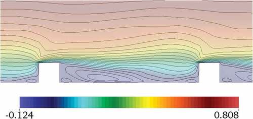
Figure 25. Skin friction coefficient for the case with ribs-like protuberances. Comparison with Dritselis & Vlachos (2011b) and Leonardi et al. (2003). Green pointed line represents the C_f value for a plane channel. Yellow Arrow represents the profile obtained in this paper. CPPE: Channel with ribs-like protuberances analyzed in this paper

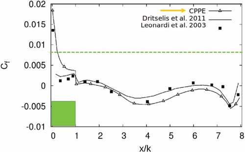
Figure 26. Streamwise mean velocity profiles normalised with Uc for the case with ribs-like protuberances. Uc is the velocity in the central line of the channel. Comparison with Dritselis (2014) and (rlandi et al. (2006). CPPE SP: Profile taken over the perturbation. CPPE EP: Profile taken between perturbations

Figure 27. Velocity fluctuations behaviour. Profiles normalised with U_b for the case with ribs-like protuberances. Comparison with Dritselis (2014) and Orlandi et al. (2006). CPPE EP: Profile taken between perturbations

Figure 28. Q-Coherent structures for a smooth-wall channel channel

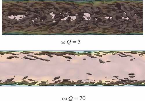
Figure 29. Q-Coherent structures for a channel with ribs-like protuberances

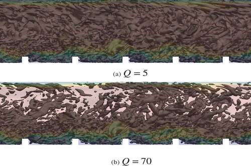
Figure 30. Streamlines for the case with cavity-like perturbations

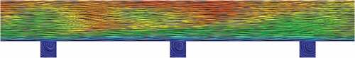
Figure 31. Streamwise mean velocity profile normalised with Uc for the case with cavity-like perturbations. Uc is the velocity in the central line of the channel. Comparison with results obtained with our implementation of the coherent structure SGS model for a plane channel

Figure 32. Velocity fluctuations behaviour. Profiles normalised with U_b for the case with cavity-like perturbations. CPNE EP: Profile taken between perturbations; CPNE SP: Profile taken above perturbations. Comparison with results obtained with our implementation of the coherent structure SGS model for a plane channel

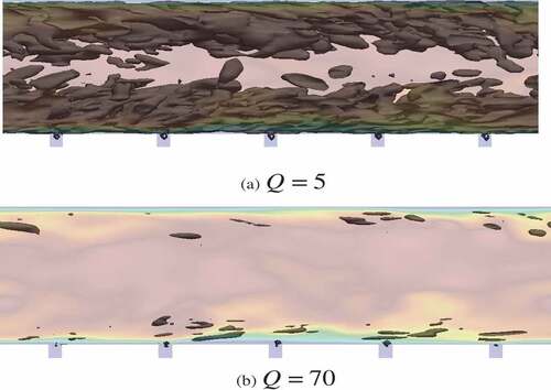
Figure 33. Q Coherent structures for the case with cavity-like perturbations

Fran, C. K., & Bogey, C. (2015). Large-eddy simulation of turbulent channel flow using relaxation filtering: Resolution requirement and Reynolds number effects. Computers & Fluids, 116, 17–28. doi:10.1016/j.compfluid.2015.03.026

 Web of Science ®Google Scholar

Viazzo, S., Dejoan, A., & Schiestel, R. (2001). Spectral features of the wall-pressure fluctuations in turbulent wall flows with and without perturba- tions using LES. International Journal of Heat and Fluid Flow, 22(1), 39–52. doi:10.1016/S0142-727X(00)00074-6

 Web of Science ®Google Scholar

Gloerfelt, X., & Berland, J. (2013). Turbulent boundary-layer noise: Direct radiation at mach number 0.5. Journal of Fluid Mechanics, 723, 318–351. doi:10.1017/jfm.2013.134

 Web of Science ®Google Scholar

Schlatter, P., Li, Q., Brethouwer, G., Johansson, A. V., & Henningson, D. S. (2010). Simulations of spatially evolving turbulent boundary layers up to Reθ = 4300. International Journal of Heat and Fluid Flow, 31(3), 251–261. doi:10.1016/j.ijheatfluidflow.2009.12.011

 Web of Science ®Google Scholar

Kim, J., Moin, P., & Moser, R. (1987). Turbulence statistics in fully de- veloped channel flow at low Reynolds number. Journal of Fluid Mechanics, 177, 133–166. doi:10.1017/S0022112087000892

 Web of Science ®Google Scholar

Moser, R. D., Kim, J., & Mansour, N. N. (1999). Direct numerical simulation of turbulent channel flow up to Re τ = 590. Physics of Fluids, 11(4), 943–945. doi:10.1063/1.869966

 Web of Science ®Google Scholar

Del A´lamo, J. C., Jimnez, J., Zandonade, P., & Moser, R. D. (2004). Scaling of the energy spectra of turbulent channels. Journal of Fluid Mechanics, 500, 135–144. doi:10.1017/S002211200300733X

 Web of Science ®Google Scholar

Zhiwei, H., Morfey, C. L., & Sandham, N. D. (2006). Wall pressure and shear stress spectra from direct simulations of channel flow. AIAA Journal, 44(7), 1541–1549. doi:10.2514/1.17638

 Web of Science ®Google Scholar

Lee, M., & Moser, R. D. (2015). Direct numerical simulation of turbulent channel flow up to Reτ approx 5200. Journal of Fluid Mechanics, 774, 395–415. doi:10.1017/jfm.2015.268

 Web of Science ®Google Scholar

Bose, S. T., Moin, P., & You, D. (2010). Grid-independent large-eddy simulation using explicit filtering. Physics of Fluids, 22(10), 105103. doi:10.1063/1.3485774

 Web of Science ®Google Scholar

Islam Mallik, M. S., Uddin, M. A., & Meah, M. A. (2014). Large eddy simulation of turbulent channel flow at Reτ = 590. IOSR–Journal of Math- Ematics, 10(6), 41–50. doi:10.9790/5728

 Google Scholar

Dritselis, C. D., & Vlachos, N. S. (2011b). Numerical investigation of momentum exchange between particles and coherent structures in low Re turbulent channel flow. Physics of Fluids, 23(2), 025103. doi:10.1063/1.3553292

 Web of Science ®Google Scholar

Leonardi, S., Orlandi, P., Smalley, R. J., Djenidi, L., & Antonia, R. A. (2003). Direct numerical simulations of turbulent channel flow with transverse square bars on one wall. Journal of Fluid Mechanics, 491, 229–238. doi:10.1017/S0022112003005500

 Web of Science ®Google Scholar

Dritselis, C. D. (2014). Large eddy simulation of turbulent channel flow with transverse roughness elements on one wall. International Journal of Heat and Fluid Flow, 50, 225–239. doi:10.1016/j.ijheatfluidflow.2014.08.008

 Web of Science ®Google Scholar

Orlandi, P., Leonardi, S., & Antonia, R. A. (2006). Turbulent channel flow with either transverse or longitudinal roughness elements on one wall. Journal of Fluid Mechanics, 561, 279–305. doi:10.1017/S0022112006000723

 Web of Science ®Google Scholar

Data availability

https://drive.google.com/drive/folders/1gezLGzKoOh1JMxsQvAiAxYUSzr5Kdtc2?usp=sharing