
Figures & data
Table 1. Real system data
Figure 1. Single-line diagram.
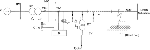
Figure 2. Wooden pole overhead line & pole mounted (11/0.4 kV) DT distribution transformer in desert region.
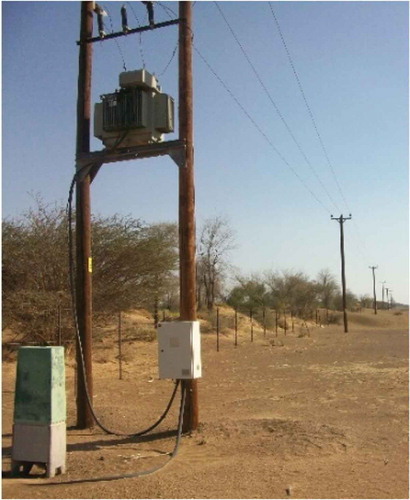
Figure 3. Representation of neutral current and voltage.
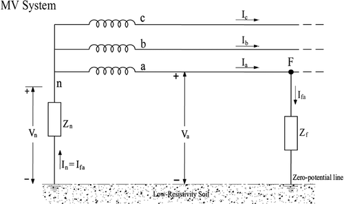
Figure 4. Flowchart for sensitivity analysis of high impedance ground fault.
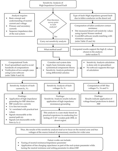
Figure 5. Simplified single-line diagram.
Table 2. Sequence impedance data of the real system
Figure 6. Magnitude of calculated fault current (Ifa) for Zf = 0.1 to 1000 Ω for different “Zn”. Graph is drawn omitting “θ” (key values are in Table ).
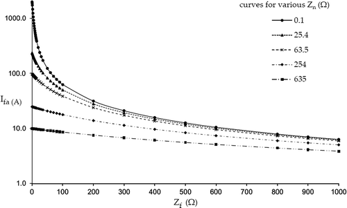
Table 3. Calculated fault currents for different neutral earthing and fault impedances
Figure 7. Recorded voltage and current waveforms for case—1. (Field-measured values are in Table ).
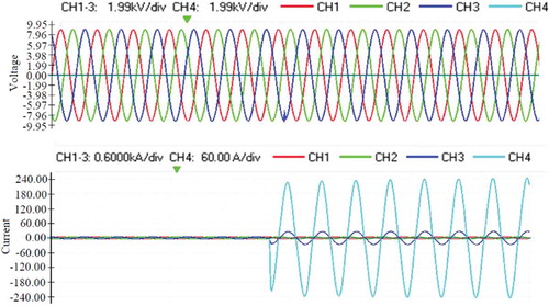
Figure 8. Recorded voltage and current waveforms for case—2. (Field-measured values are in Table ).
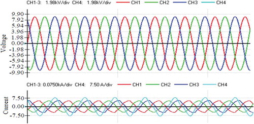
Figure 9. Recorded voltage and current waveforms for case—3. (Field-measured values are in Table ).
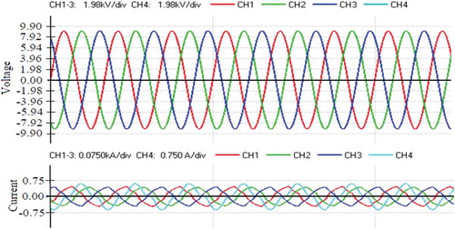
Table 4. Field measured values for case—1, 2 and 3
Figure 10. Magnitude of the line voltage (Vb) for Zf = 0.1 to 1000 Ω for different Zn values. Graph is drawn omitting “θ”.
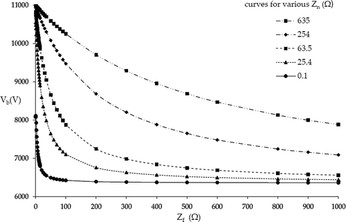
Figure 11. Magnitude of the line voltage (Vc) for Zf = 0.1 to 1000 Ω for different Zn values. Graph is drawn omitting “θ”.
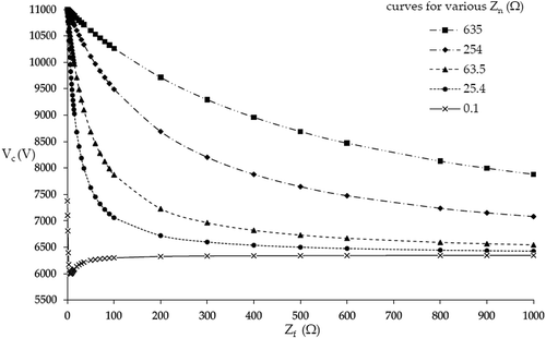
Figure 12. Magnitude of the MV bus voltage (VA) for Zf = 0.1 to 1000 Ω for different “Zn” values. Graph is drawn omitting “θ” (key values are in Table ).
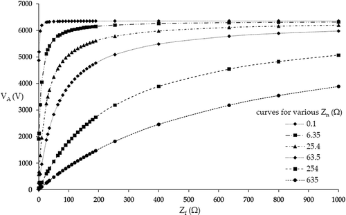
Figure 13. Magnitude of the MV bus voltage (VB) for Zf = 0.1 to 1000 Ω for different “Zn” values. Graph is drawn omitting “θ” (key values are in Table ).
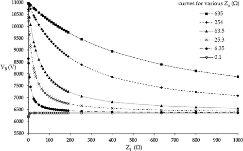
Figure 14. Magnitude of the MV bus voltage (VC) for Zf = 0.1 to 1000 Ω for different “Zn” values. Graph is drawn omitting “θ” (key values are in Table ).
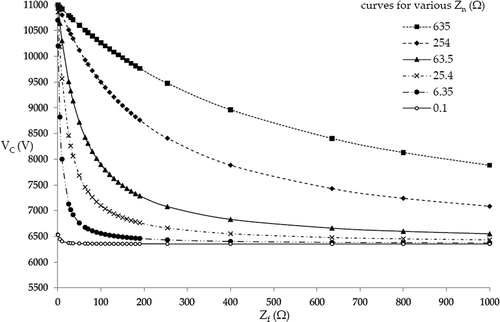
Table 5. Magnitude of MV Bus voltage (VA) for various fault impedances
Table 6. Magnitude of MV Bus voltage (VB) for various fault impedances
Table 7. Magnitude of MV Bus voltage (VC) for various fault impedances
Figure 15. Magnitude of neutral voltage (VN) for Zf = 0.1 to 1000 Ω for different “Zn” . Graph is drawn omitting “θ” (key values are in Table ).
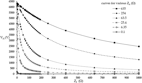
Table 8. Magnitude of neutral voltage (VN) for various fault impedances
Figure 16. Single-line diagram CYME Simulation.
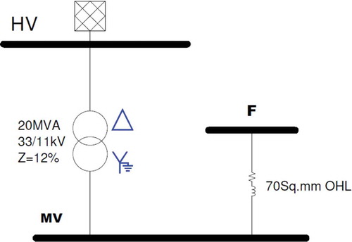
Table 9. Computational results for MV bus voltage
Table 10. Computational results for voltages at fault “F”
Figure 17. Sensitivity of fault current S(Ifa) to Zf = 0.1 to 1000 Ω for different values of “Zn”. Graph is drawn omitting “θ” (key values are in Table ).
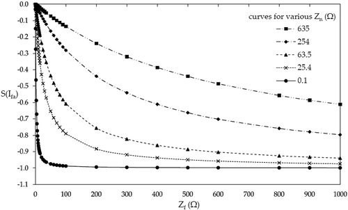
Table 11. Sensitivity of fault current S(Ifa) for different neutral earthing and fault impedances
Table 12. Sensitivity of line voltage S(Vb) for different neutral earthing and fault impedances
Table 13. Sensitivity of line voltage S(Vc) for different neutral earthing and fault impedances
Figure 18. Sensitivity of neutral voltage (VN) for different values of “Zn”. Graph is drawn omitting “θ” (key values are in Table ).

Table 14. Sensitivity of neutral voltage S(Vn) with various neutral earthing impedances
Figure 19. Representation of a fallen conductor in high-resistivity desert soil.
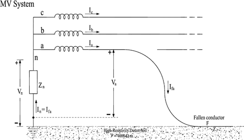
Table 15. Site-measured desert soil resistivity
Table 16. Computed contact resistance of a fallen conductor
Nomenclature