Figures & data
Figure 1. 3DCG Images of Rear Designs. Subfigures (a)-(j) were 3DCG images generated by reference to photographs of newly launched vehicle with typical tail lamp design. The images were rendered at 960 × 540 pixels in night light conditions using Autodesk Maya 2016
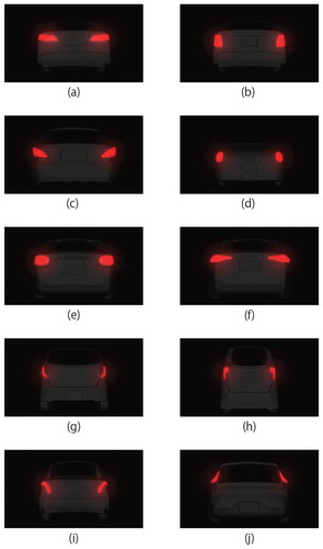
Table 1. Selected evaluation words
Figure 2. Mapping of Evaluation Words. This figure shows two-dimensional plane mapping of 49 evaluation words based on the MDS results. The x-axis is a scale of comfort (comfortable—uncomfortable) and the y-axis is a scale of activity (high—low)
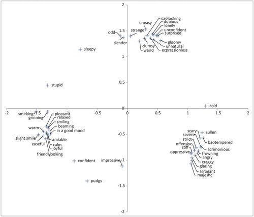
Table 2. The selected key words
Table 3. Factor analysis results (subjective evaluation experiment 1)
Figure 3. Recreated Stimulus Material. The eight designs were recreated in terms of the curvature of the tail lamps and used for the stimulus material in Test 5: Subjective Evaluation Experiment 2. Each of subfigures (a)-(h) indicates the Stimulus A-H
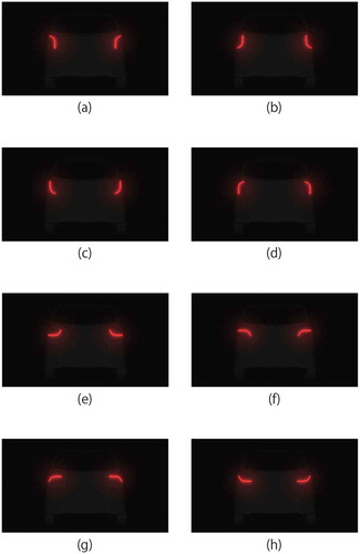
Table 4. Factor analysis results (subjective evaluation experiment 2)
Figure 4. Factor Scores for the Stimuli. The stimulus materials are mapped on two-dimensional graphs. (a) was a scatter plot with Factor 1 as the x-axis and Factor 2 as the y-axis, (b) was a scatter plot with Factor 2 as the x-axis and Factor 3 as the y-axis, (c) was a scatter plot with Factor 1 as the x-axis and Factor 3 as the y-axis
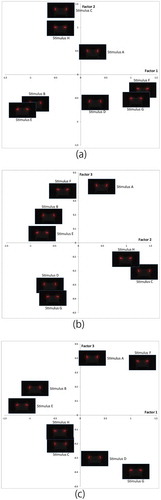
Figure 5. Differences in Impression depending on Direction of Convex Side. This figure presents a summary of how factor scores depend on direction of convex side (inward—outward and upward—downward) and aspect ratio (vertically long—horizontally long)
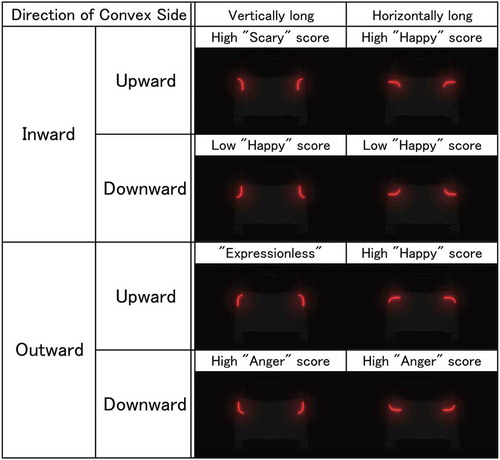
Figure 6. Visual Stimuli. Tail lamp design arrays used as stimuli in the visual search task. (a) shows a tar-get-absent stimulus, and (b) shows a target-present stimulus at bottom position, in which one of the key images is the target
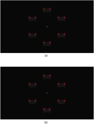
Figure 7. Experiment Procedure of Visual Search Task. Each trial of the search task consisted of a centrally presented fixation cross (500 ms), followed by the search array which remained on screen until a response was made and then a blank black screen (1500, 2000, 2500 ms)
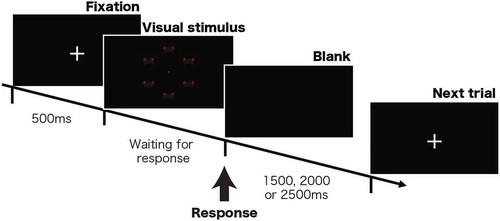
Figure 8. Response Accuracy and Response Time Results. This figure shows experiment results; response accuracy in subfigure (a) and response time in subfigure (b). With regard to response accuracy, the ANOVA did not indicate any statistically significant results for either factor. With regard to response time, the ANOVA indicated a main effect for the target type (F(1,8) = 9.74, p < .05), but not for the target position, and it did not indicate an interaction effect
Figure 9. Biosemi Electrodes Layout. 64 + 2 channel Biosemi electrodes layout. The red circles indicate the electrodes used in this study
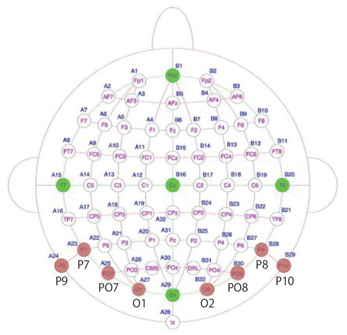
Figure 10. Grand Average ERPs. The upper section shows grand averaged ERPs elicited in the 500 ms interval in response to threatening (black lines) and friendly (gray lines) target faces, both contra-lateral (solid lines) and ipsilateral (dashed lines) to the visual hemifield where the face was presented. The shaded area represents the time window (240–300 ms) used in the analyses. The lower section shows the topographical voltage maps (top views) for threatening and friendly targets presented on the right side (left maps) and left side (right maps), showing the distribution of N2pc negativity in the time interval 240–300 ms
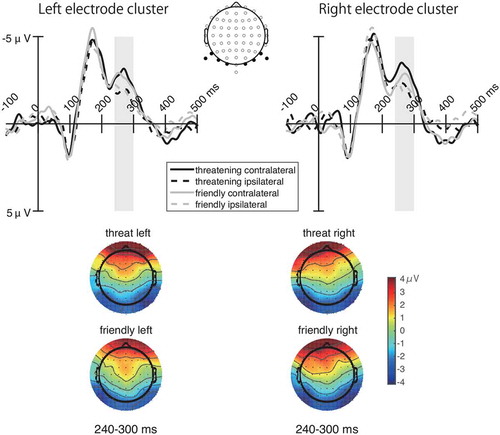
Figure 11. Comparison of the N2pc between Threatening and Friendly. Magnitude of the N2pc amplitude (contralateral minus ipsilateral)