A Statistical Technique for Modelling Dissolved Oxygen in Salt Lakes

Figures & data

Figure 1. The area of study; (a) Sawa Lake region retrieved by QGIS, and (b) Map of Sawa Lake retrieved from Landsat 8 OLI/TIRS Level-2 Data Products (WRS path/row: 168/038; acquired on 3 June 2017), showing the locations of samples used in this study

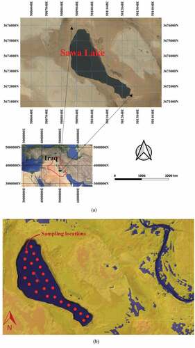
Table 1. Monthly averaged water quality parameters of Sawa Lake in 2017

Month	Jan	Feb	Mar	Apr	May	Jun	Jul	Aug	Sep	Oct	Nov	Dec
pH	8.1	8.16	8.26	8.3	8.33	8.38	8.45	8.51	8.6	8.55	8.34	8.21
DO (mg/L)	8.5	8.46	8.4	8.37	8.33	8.3	8.2	7.9	8	8.1	8.38	8.44
TDS (mg/L)	26,240	26,248	26,263	26,290	26,301	26,320	26,550	26,640	26,600	26,590	26,280	26,250
TSS (mg/L)	115	118	120	121	123	125	128	130	133	127	125	116
SO4 (mg/L)	6450	6530	6562	6570	6610	6689	6730	6800	6780	6700	6620	6480
Cl (mg/L)	8445	8476	8488	8495	8525	8620	8659	8750	8710	8640	8530	8455
NO3 (mg/L)	7.1	7.2	7.4	7.6	7.76	8.29	9.18	9.5	9.1	8.3	8.1	7.3
Ca (mg/L)	1890	1894	1901	1910	1918	1926	1933	1935	1924	1921	1908	1895
Mg (mg/L)	1805	1800	1801	1820	1837	1844	1848	1850	1851	1834	1832	1820
Na (mg/L)	3710	3698	3770	3790	3799	3840	3870	3900	3830	3801	3780	3720
EC (µS/cm)	38,110	38,011	38,062	38,310	38,520	38,690	38,710	38,890	38,820	38,609	38,587	38,240
F (mg/L)	4.9	5	5	5.2	5.23	5.4	5.7	6	5.2	5.1	5	4.8
k (mg/L)	419	422	425	434	439	444	450	459	451	439	431	420
Turb (mg/L)	28	29	22	26	29	31	33	35	32	31	30	29
Temp (C)	6	15	21.4	25	30	33	39	42	37	23	19	7
T.H (mg/L)	12,199	12,307	12,500	12,555	12,708	12,890	12,920	12,990	12,490	12,379	12,236	12,220

Figure 2. Statistical conceptual model

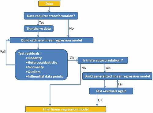
Figure 3. Correlation plots (a, b, and c) of Sawa Lake data; (a) Scatterplot matrix of Sawa Lake data, (b) Correlation color matrix of Sawa Lake data, and (c) Correlation pie plots of Sawa Lake data

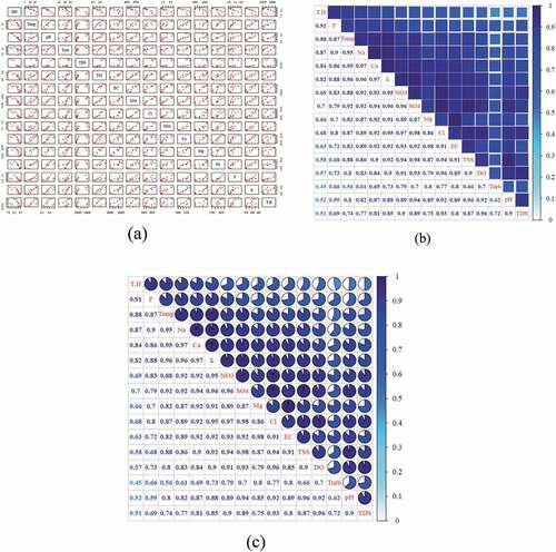
Figure 4. Boxplots and correlation matrix of dissolved oxygen, temperature, and turbidity in 2017 extracted from Sawa Lake raw data; (a) Dissolved oxygen, temperature, and turbidity boxplots from Sawa Lake data in 2017, and b) Dissolved oxygen, temperature, and turbidity correlation matrix from Sawa Lake data in 2017

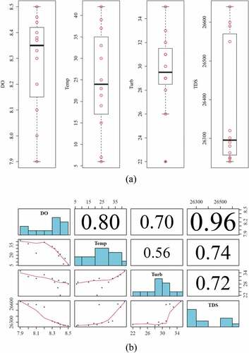
Table 2. The full linear regression model summary statistics of equation 1(1) $DO=e^{\left[2.47520-0.01997logTemp-0.08883logTurb\right]}$(1)

Residuals ———— Min 1^st Quantile Median 3^rd Quantile Max -0.0178968 − 0.0123502 − 0.0001187 0.0119282 0.0159006 Coefficients ————— Estimate Standard error t-value Pr(>|t|) (Intercept) 2.475199 0.124297 19.914 9.43e-09 logTemp −0.019967 0.007319 − 2.728 0.0233 logTurb −0.088826 0.038717 − 2.294 0.0474 ————————————————————————– Residual standard error: 0.01431 on 9 degrees of freedom Multiple R-squared: 0.6925,Adjusted R-squared: 0.6242 F-statistic: 10.14 on 2 and 9 DF, p-value: 0.004956

Table 3. The full linear regression model summary statistics of equation 2(2) $DO=e^{\left[39.4915-3.6715logTDS\right]}$(2)

Residuals ———— Min 1^st Quantile Median 3^rd Quantile Max -0.011001 − 0.004209 − 0.001864 0.003958 0.013846 Coefficients ————— Estimate Standard error t value Pr(>|t|) (Intercept) 39.4915 3.5854 11.02 6.51e-07 logTDS −3.6715 0.3522 − 10.43 1.08e-06 ————————————————————————– Residual standard error: 0.007107 on 10 degrees of freedom Multiple R-squared: 0.9157,Adjusted R-squared: 0.9073 F-statistic: 108.7 on 1 and 10 DF, p-value: 1.084e-06

Figure 5. Linear regression validation graphs; (a) Model validation graphs of .Eq. 1(1) $DO=e^{\left[2.47520-0.01997logTemp-0.08883logTurb\right]}$(1) , and (b) Model validation graphs of Eq. 2(2) $DO=e^{\left[39.4915-3.6715logTDS\right]}$(2)

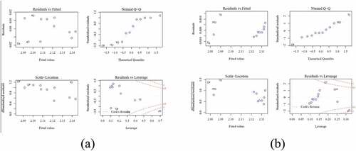
Table 4. Regression models and summary statistics

Model	R-squared	p-value	Shaprio-Wilk test w-value p-value	Equal variance F-test p-value
Eq. 1(1) $DO=e^{\left[2.47520-0.01997logTemp-0.08883logTurb\right]}$(1)	0.6242	0.004956	0.8744 0.07427	0.2641
Eq. 2(2) $DO=e^{\left[39.4915-3.6715logTDS\right]}$(2)	0.9073	1.08E-06	0.9653 0.8554	0.05062

Figure 6. Model auto-correlation plots

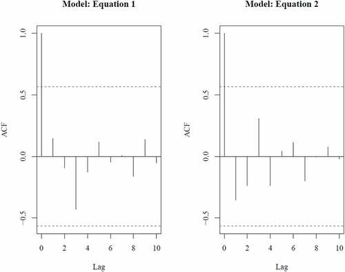
Figure 7. Comparisons between the model predictions with raw data; (a) DO in Sawa Lake by fitting the model of Eq. 2(2) $DO=e^{\left[39.4915-3.6715logTDS\right]}$(2) to the raw data in 2017, and (b) The interaction among dissolved oxygen, temperature, and turbidity, the circle size was scaled by the relevant temperature

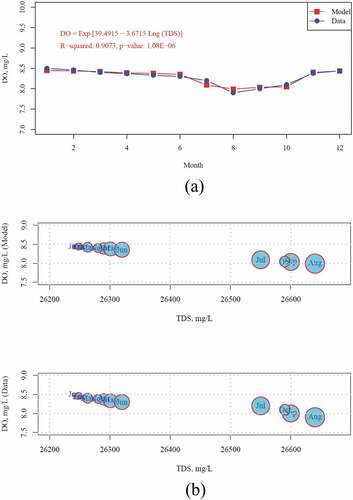
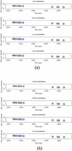
Figure 8. The contribution of ionic compounds (a-h) to TDS and how they impact DO, the circle size was scaled by the relevant ion concentration