Performance analysis of downlink massive MIMO system with precoding techniques and pilot reuse factor

Figures & data

Figure 1. Multi-Cell Multi-user Downlink TDD-Massive MIMO System Model.

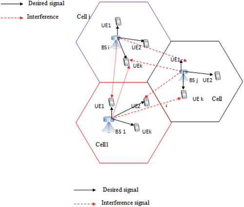
Figure 2. NLOS propagation under local scattering spatial correlation model (Bjornson et al., 2017).

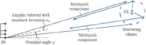
Figure 3. Uplink Pilot Contamination in a multi cell scenario where BS i in cell i receive pilots from adjacent cell (Zhao et al., 2017).

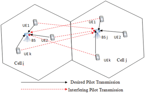
Figure 4. Block diagram representation of a multi-cell DL Ma-MIMO system with linear precoding (Marzetta & Quoc Ngo, 2016).

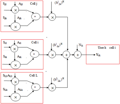
Table 1. Parameters and values

parameters	values (considerations)
Number of cells	Multi-cells ((Marzetta, 2010; Quoc Ngo, 2015))
Cell radius	1000m
Channel state information	Perfect and imperfect CSI at the BS
Channel model	Correlated Rayleigh fading
Number of antennas per BS (Fixed)	100 (Salh & Audah, 2020)
Range of antennas per BS (When varied)	10–110
Number of users (Fixed)	10 (Salh & Audah, 2020)
Number of users(Varied)	0–40 (Thakur & Chandra Mishra, 2019)
UL and DL power	20dBm (Bjornson et al., 2017)
PRF	1,3,4
Channel gain at 1 km $(\mathrm{{\rm Y}})$	148.1 dB (Bjornson et al., 2017)
Path-loss exponent $(\mathit{\alpha })$	3.76 (Marzetta, 2010)
Receiver noise power	94 dBm (Bjornson et al., 2017)
Bandwidth	20MHz (Marzetta & Quoc Ngo, 2016)
Carrier frequency	2GHz (Marzetta & Quoc Ngo, 2016)
Coherence interval	300 (Marzetta & Quoc Ngo, 2016)
Number of channel realizations	100
Shadow fading standard deviation $({\sigma }_{\mathit{sf}})$	10dB (Marzetta, 2010)

Figure 5. Average sum SE with respect to the number of BS antennas for M-MMSE, ZF and MRT precoding techniques (for a PRF of one, three and four and K=10).

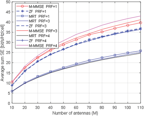
Figure 6. Average sum SE with respect to the number of BS antennas for M-MMSE, ZF and MRT precoding techniques (for a PRF of one and M=100).

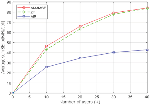
Figure 7. Average sum SE with respect to the number of users for M-MMSE, ZF and MRT. Precoding techniques (for a PRF of three and M=100).

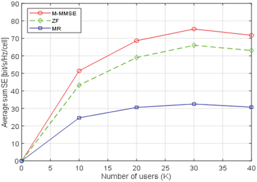
Figure 8. Average sum SE with respect to the number of users for M-MMSE, ZF and MRT. Precoding techniques (for a PRF of four and M=100).

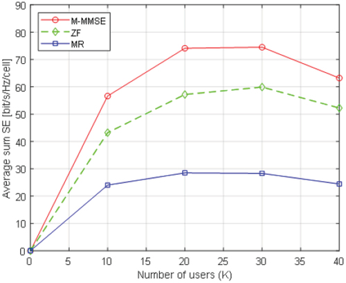
Figure 9. Average sum SE with respect to the number of Antennas for MMSE, ZF and MRT precoding techniques with perfect and imperfect CSI (PRF of one) and K = 10.

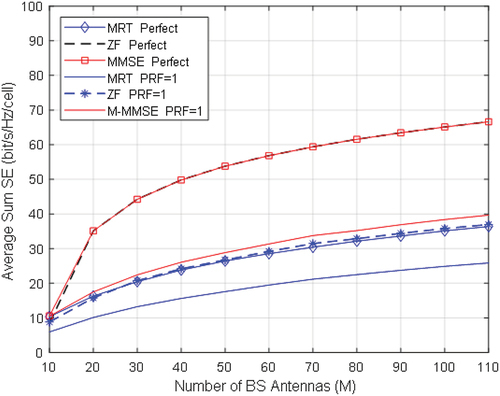
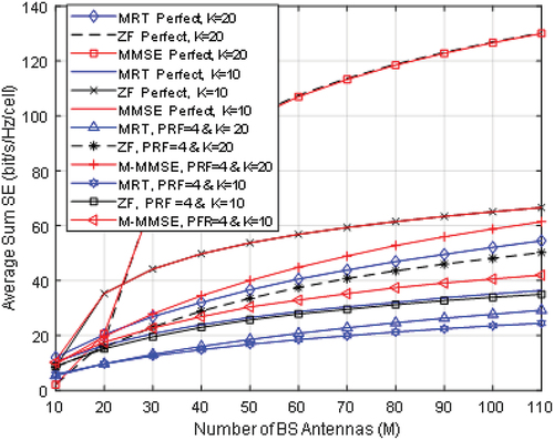
Figure 10. Average sum SE with respect to the number of Antennas for MMSE,ZF and MRT precoding techniques with perfect and imperfect act CSI (PRF of four) and K = 10, K = 20.

Bjornson, E., Hoydis, J., & Sanguinetti, L. (2017). Massive MIMO networks: Spectral, energy, and hardware efficiency. Foundations and Trends in Signal Processing, 11(3–4), 154–655. https://doi.org/10.1561/2000000093

 Web of Science ®Google Scholar

Zhao, M., Zhang, H., Guo, S., & Yuan, D. (2017). Joint pilot assignment and pilot contamination precoding design for massive MIMO systems. Proceedings of the 2017 26th Wireless and Optical Communication Conference (WOCC), 1–6. https://doi.org/10.1109/WOCC.2017.7929001

 Google Scholar

Marzetta, T. L., & Quoc Ngo, H. (2016). Fundamentals of massive MIMO. Cambridge University Press.

 Google Scholar

Marzetta, T. L. (2010). Noncooperative cellular wireless with unlimited numbers of base station antennas. IEEE Transactions on Wireless Communications, 9(11), 3590–3600. https://doi.org/10.1109/TWC.2010.092810.091092

 Web of Science ®Google Scholar

Quoc Ngo, H. (2015). Massive MIMO: Fundamentals and system designs, volume 1642. Linkoping University Electronic Press.

 Google Scholar

Salh, A., & Audah, L. (2020). Nor shahida mohd shah, and shipun anuar hamzah. mitigating pilot contamination for channel estimation in multi-cell massive MIMO systems. Wireless Personal Communications, 112(3), 1643–1658. https://doi.org/10.1007/s11277-020-07120-9

 Web of Science ®Google Scholar

Thakur, A., & Chandra Mishra, R. (2019). Performance analysis of energy efficient multi-cell massive MIMO system. Proceedings of the 2019 10th International Conference on Computing, Communication and Networking Technologies (ICCCNT), 1–7. https://doi.org/10.1109/ICCCNT45670.2019.8944389

 Google Scholar