A new Bell-exponential model: Properties and applications

Figures & data

Figure 1. Graphical illustration of PDF for some parametric values.

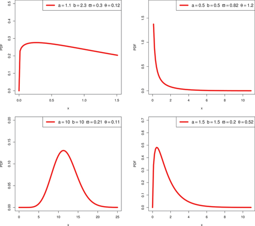
Figure 2. Graphical illustration of HRF for some parametric values.

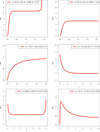
Figure 3. Graphical illustration of mean and variance of the KwBE distribution for $a\in (1.5:5.5)$, $\theta =1$, $b=7$ and $\varpi \in (0.10:5.0)$.

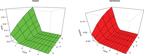
Figure 4. Graphical illustration of mean and variance of the KwBE distribution for $a=5$, $\theta =1$, $b\in (1.5:5.5)$ and $\varpi \in (0.10:5.0)$.

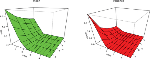
Figure 5. Graphical illustration of skewness and kurtosis of the KwBE distribution for $a\in (5:30)$, $\theta =0.20$, $b=2$ and $\varpi \in (0.50:2.0)$.

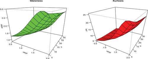
Figure 6. Graphical illustration of skewness and kurtosis of the KwBE distribution for $a=7$, $\theta =0.30$, $b\in (3:6)$ and $\varpi \in (0.50:2.0)$.

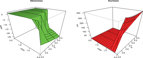
Figure 7. Plot of RE for some parametric values.

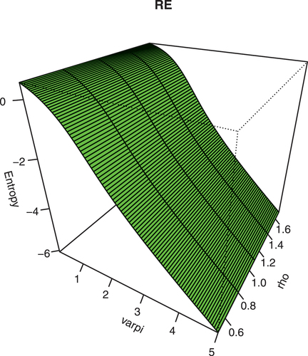
Figure 8. Graphical illustration of biases at varying sample sizes.

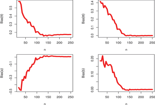
Figure 9. Graphical illustration of MSEs at varying sample sizes.

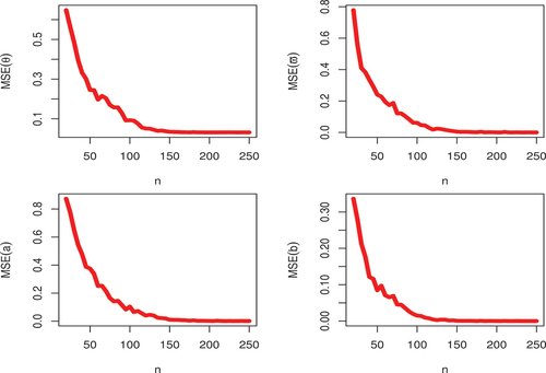
Table 1. Proposed GASP based on the KwBE model

$r_2$	2	4	6	8
$n$	–	100	50	30
$g$	–	10	5	3
$c$	–	5	4	3
$P(a)$	–	0.9688	0.9803	0.9838

Table 2. A GASP under the KwBE model, $a=1.00$, $b=1.00$, $\varpi =1.25$

	$\mathit{r}\mathbf{=}\mathbf{5}$							$\mathit{r}\mathbf{=}\mathbf{10}$
		${\mathit{a}}_{\mathbf{1}}\mathbf{=}\mathbf{0.5}$			${\mathit{a}}_{\mathbf{1}}\mathbf{=}\mathbf{5}$			${\mathit{a}}_{\mathbf{1}}\mathbf{=}\mathbf{0.5}$			${\mathit{a}}_{\mathbf{1}}\mathbf{=}\mathbf{1}$
$\beta$	${\mathit{r}}_{\mathbf{2}}$	$\mathit{g}$	$\mathit{c}$	$\mathit{p}(a)$	$\mathit{g}$	$\mathit{c}$	$\mathit{p}(a)$	$\mathit{g}$	$\mathit{c}$	$p(a)$	$\mathit{g}$	$\mathit{c}$	$\mathit{p}(a)$
0.25	2	–	–	–	–	–	–	–	–	–	–	–	–
	4	40	3	0.9860	7	3	0.9721	3	3	0.9701	2	4	0.9624
	6	8	2	0.9815	3	2	0.9559	2	2	0.9565	1	3	0.9748
	8	8	2	0.9917	3	2	0.979	2	2	0.9792	1	3	0.9899
0.1	2	–	–	–	–	–	–	–	–	–	–	–	–
	4	66	3	0.9770	12	3	0.9527	5	3	0.9507	5	5	0.9843
	6	12	2	0.9724	12	3	0.9881	5	3	0.9875	2	3	0.9503
	8	12	2	0.9875	4	2	0.9721	3	2	0.9689	2	3	0.9800
0.05	2	–	–	–	–	–	–	–	–	–	–	–	–
	4	85	3	0.9705	95	4	0.9845	17	3	0.9798	7	5	0.9781
	6	16	2	0.9633	15	3	0.9852	7	3	0.9825	2	3	0.9503
	8	16	2	0.9834	5	2	0.9652	3	2	0.9689	2	3	0.9800
0.01	2	–	–	–	–	–	–	–	–	–	–	–	–
	4	131	3	0.9549	146	4	0.9763	26	4	0.9693	10	5	0.9688
	6	131	3	0.9899	23	3	0.9774	10	3	0.9751	5	4	0.9803
	8	24	2	0.9752	7	2	0.9517	10	3	0.991	3	3	0.9838

Remark: Hyphens (–) are inserted in required cells for a large sample size.

Table 3. A GASP under the KwBE model, $a=1.00$, $b=1.00$, $\varpi =1.50$

	$\mathit{r}\mathbf{=}\mathbf{5}$							$\mathit{r}\mathbf{=}\mathbf{10}$
		$\mathit{r}\mathbf{=}\mathbf{5}$			$\mathit{r}\mathbf{=}\mathbf{10}$			${\mathit{a}}_{\mathbf{1}}\mathbf{=}\mathbf{0.5}$			${\mathit{a}}_{\mathbf{1}}\mathbf{=}\mathbf{5}$
$\beta$	${\mathit{r}}_{\mathbf{2}}$	$\mathit{g}$	$\mathit{c}$	$\mathit{p}(a)$	$\mathit{g}$	$\mathit{c}$	$\mathit{p}(a)$	$\mathit{g}$	$\mathit{c}$	$p(a)$	$\mathit{g}$	$\mathit{c}$	$\mathit{p}(a)$
0.25	2	–	–	–	–	–	–	–	–	–	–	–	–
	4	41	3	0.9866	7	3	0.9735	3	3	0.9718	2	4	0.9644
	6	8	2	0.9824	3	2	0.9578	2	2	0.9584	1	3	0.9761
	8	8	2	0.9921	3	2	0.9800	2	2	0.9802	1	3	0.9905
0.1	2	–	–	–	–	–	–	–	–	–	–	–	–
	4	68	3	0.9779	12	3	0.9550	5	3	0.9535	5	5	0.9854
	6	13	2	0.9715	12	3	0.9888	5	3	0.9883	2	3	0.9528
	8	13	2	0.9872	4	2	0.9734	3	2	0.9705	2	3	0.9811
0.05	2	–	–	–	–	–	–	–	–	–	–	–	–
	4	88	3	0.9715	95	4	0.9855	17	4	0.9814	7	5	0.9796
	6	16	2	0.9651	15	3	0.9861	7	3	0.9836	2	3	0.9528
	8	16	2	0.9843	5	2	0.9669	3	2	0.9705	2	3	0.9811
0.01	2	–	–	–	–	–	–	–	–	–	–	–	–
	4	135	3	0.9565	146	4	0.9778	26	4	0.9716	10	5	0.9709
	6	135	3	0.9903	23	3	0.9787	10	3	0.9767	5	4	0.9816
	8	25	2	0.9755	7	2	0.9540	5	2	0.9513	3	3	0.9718

Remark: Hyphens (–) are inserted in required cells for a large sample size.

Table 4. Descriptive information of both data sets

Data	$\mathit{n}$	${\mathit{x}}_{\mathbf{0}}$	${\mathit{Q}}_{\mathbf{1}}$	$\tilde{\mathit{x}}$	$\bar{\mathit{x}}$	$\sigma$	${\mathit{Q}}_{\mathbf{3}}$	${\mathit{x}}_{\mathit{m}}$	S	K
First	50	0.040	0.390	1.190	1.975	2.116	3.078	7.490	1.325	3.803
Second	188	1.000	20.750	54.000	92.070	107.916	118.000	603.000	2.139	8.023

Figure 10. Graphical illustration of first (top) and second (bottom) data.

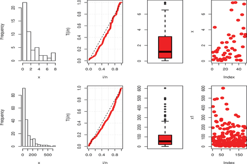
Figure 11. Graphical illustration of the estimated PDF and the CDF under the KwBE model, first (top) and second (bottom) data.

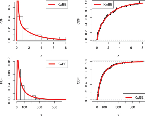
Table 5. The fitted models along with goodness-of-fit statistics, MLEs and S.E, first data

Model	-2$\hat{\mathrm{\ell }}$	$A^{\ast }$	$W^{\ast }$	KS	PV	Param.	Esti.	S.E
KwBE	81.02807	0.16211	0.01786	0.04531	1.000	$\hat{\theta }$	3.4481	0.1420
						$\hat{\varpi }$	1.5202	0.0738
						$\hat{a}$	4.4080	0.5467
						$\hat{b}$	0.1231	0.0169
KwPE	81.38482	0.18024	0.01945	0.05557	0.998	$\hat{\theta }$	3.7937	0.0517
						$\hat{\lambda }$	4.0342	0.0476
						$\hat{a}$	2.6302	0.0963
						$\hat{b}$	0.1135	0.0161
EE	83.37585	0.32787	0.03661	0.06695	0.979	$\hat{\alpha }$	0.4428	0.0867
						$\hat{\beta }$	0.8173	0.1462
MOE	83.22806	0.30430	0.03361	0.07476	0.943	$\hat{\alpha }$	0.3699	0.1262
						$\hat{a}$	0.5363	0.2806
EW	83.33341	0.30996	0.03409	0.06936	0.970	$\hat{\alpha }$	0.6359	0.7354
						$\hat{\beta }$	0.8410	0.4945
						$\hat{a}$	1.0785	1.0673
OWE	83.06346	0.33346	0.03721	0.05837	0.996	$\hat{\alpha }$	0.1029	0.1444
						$\hat{a}$	3.2647	4.8481
						$\hat{b}$	0.7906	0.1479
KE	83.89684	0.35807	0.04111	0.08956	0.817	$\hat{\alpha }$	3.9617	0.0607
						$\hat{a}$	0.8248	0.0488
						$\hat{b}$	0.1249	0.0178
BE	83.37565	0.32757	0.03657	0.06692	0.979	$\hat{\alpha }$	0.4098	1.9573
						$\hat{a}$	0.8178	0.1537
						$\hat{b}$	1.0773	4.9595
TLE	83.37585	0.32787	0.03661	0.06692	0.979	$\hat{\alpha }$	0.2214	0.0433
						$\hat{a}$	0.8172	0.1462
APEE	83.24683	0.30599	0.03347	0.06789	0.975	$\hat{\alpha }$	0.3978	0.1293
						$\hat{\gamma }$	0.5276	0.6801
						$\hat{\beta }$	0.8926	0.1971
TEE	83.29617	0.03444	0.31303	0.06753	0.977	$\hat{\alpha }$	0.4135	0.1203
						$\hat{\lambda }$	0.1942	0.4893
						$\hat{\beta }$	0.8606	0.1711
GEE	83.37542	0.32727	0.03652	0.06692	0.979	$\hat{\alpha }$	0.4377	0.1934
						$\hat{\beta }$	0.8473	1.0657
						$\hat{\lambda }$	0.9662	1.1465
EEP	83.24683	0.305995	0.03347	0.06788	0.975	$\hat{\alpha }$	0.3978	0.1293
						$\hat{\beta }$	0.8926	0.1972
						$\hat{\lambda }$	0.6388	1.2890
W	83.33635	0.31258	0.03442	0.06832	0.974	$\hat{\alpha }$	0.5812	0.1035
						$\hat{\beta }$	0.8792	0.0984
NH	83.48003	0.31746	0.03543	0.07885	0.915	$\hat{\alpha }$	0.9466	0.7005
						$\hat{\beta }$	0.5490	0.2112

Table 6. The fitted models along with goodness-of-fit statistics, MLEs and S.E, second data

Model	-2$\hat{\mathrm{\ell }}$	$A^{\ast }$	$W^{\ast }$	KS	PV	Param.	Esti.	S.E
KwBE	1031.748	0.16072	0.02027	0.03131	0.993	$\hat{\theta }$	0.0179	0.0082
						$\hat{\varpi }$	1.0624	0.2063
						$\hat{a}$	1.7971	0.4837
						$\hat{b}$	0.4429	0.1629
KwPE	1032.529	0.27743	0.03912	0.04150	0.903	$\hat{\theta }$	0.0124	0.0071
						$\hat{\lambda }$	2.2214	0.9222
						$\hat{a}$	1.3129	0.3032
						$\hat{b}$	0.6232	0.3235
EE	1037.75	1.20421	0.19422	0.07211	0.282	$\hat{\alpha }$	0.0102	0.0010
						$\hat{\beta }$	0.9109	0.0864
MOE	1034.747	0.55861	0.08571	0.05506	0.619	$\hat{\alpha }$	0.0077	0.0013
						$\hat{a}$	0.5225	0.1316
EW	1033.148	0.03638	0.27286	0.04499	0.841	$\hat{\alpha }$	0.2114	0.1612
						$\hat{\beta }$	0.5182	0.1170
						$\hat{a}$	3.2556	1.6762
OWE	1041.214	1.67031	0.27130	0.07734	0.211	$\hat{\alpha }$	0.0023	0.0002
						$\hat{a}$	2.9541	0.3688
						$\hat{b}$	0.7821	0.0429
KE	1037.775	1.20570	0.19447	0.07376	0.258	$\hat{\alpha }$	0.0108	0.0058
						$\hat{a}$	0.9150	0.0883
						$\hat{b}$	0.9519	0.4929
BE	1037.815	1.21304	0.19572	0.07389	0.256	$\hat{\alpha }$	0.0132	0.0083
						$\hat{a}$	0.9130	0.0892
						$\hat{b}$	0.7805	0.4811
TLE	1037.772	1.20787	0.19482	0.07050	0.308	$\hat{\alpha }$	0.0052	0.0005
						$\hat{a}$	0.9221	0.0865
APEE	1034.066	0.50873	0.07673	0.04981	0.739	$\hat{\alpha }$	0.0072	0.0014
						$\hat{\gamma }$	0.1422	0.1032
						$\hat{\beta }$	1.1146	0.0951
TEE	1035.506	0.79634	0.12540	0.05320	0.662	$\hat{\alpha }$	0.0084	0.0014
						$\hat{\lambda }$	0.4918	0.2173
						$\hat{\beta }$	1.0033	0.0875
GEE	1038.036	1.23954	0.20018	0.06815	0.347	$\hat{\alpha }$	0.0102	0.0014
						$\hat{\beta }$	0.7932	0.2346
						$\hat{\lambda }$	1.0877	0.2889
EEP	1034.06	0.50628	0.07629	0.04951	0.746	$\hat{\alpha }$	0.0071	0.0015
						$\hat{\beta }$	1.1147	0.0951
						$\hat{\lambda }$	1.9853	0.7620
W	1036.751	0.99738	0.15948	0.05707	0.573	$\hat{\alpha }$	0.0170	0.0043
						$\hat{\beta }$	0.9111	0.0485
NH	1034.997	0.58898	0.09054	0.05168	0.697	$\hat{\alpha }$	0.0208	0.0051
						$\hat{\beta }$	0.6931	0.0883

Table 7. A GASP based on the KwBE model, $a=4.4080$, $b=0.1231$, $\varpi =1.5202$, first data

	$\mathit{r}\mathbf{=}\mathbf{5}$							$\mathit{r}\mathbf{=}\mathbf{10}$
		${\mathit{a}}_{\mathbf{1}}\mathbf{=}\mathbf{0.5}$			${\mathit{a}}_{\mathbf{1}}\mathbf{=}\mathbf{5}$			${\mathit{a}}_{\mathbf{1}}\mathbf{=}\mathbf{0.5}$			${\mathit{a}}_{\mathbf{1}}\mathbf{=}\mathbf{1}$
$\beta$	${\mathit{r}}_{\mathbf{2}}$	$\mathit{g}$	$\mathit{c}$	$\mathit{p}(a)$	$\mathit{g}$	$\mathit{c}$	$\mathit{p}(a)$	$\mathit{g}$	$\mathit{c}$	$p(a)$	$\mathit{g}$	$\mathit{c}$	$\mathit{p}(a)$
0.25	2	–	–	–	–	–	–	–	–	–	–	–	–
	4	27	3	0.9801	44	4	0.9778	6	4	0.983	2	2	0.9695
	6	6	2	0.9850	7	3	0.9827	2	2	0.9535	1	1	0.9778
	8	2	1	0.9704	3	2	0.9641	2	2	0.9874	1	0	0.9804
0.1	2	–	–	–	–	–	–	–	–	–	–	–	–
	4	44	3	0.9678	73	4	0.9635	9	4	0.9746	–	–	–
	6	9	2	0.9777	12	3	0.9706	2	2	0.9535	3	4	0.9669
	8	3	1	0.9560	4	2	0.9524	2	2	0.9874	2	3	0.9612
0.05	2	–	–	–	–	–	–	–	–	–	–	–	–
	4	57	3	0.9585	95	4	0.9527	11	4	0.9691	–	–	–
	6	12	2	0.9703	15	3	0.9634	5	3	0.9863	4	4	0.9562
	8	12	2	0.9927	15	3	0.9889	3	2	0.9812	2	3	0.9612
0.01	2	–	–	–	–	–	–	–	–	–	–	–	–
	4	934	4	0.9829	–	–	–	17	4	0.9526	–	–	–
	6	18	2	0.9558	146	4	0.9873	8	3	0.9782	10	5	0.9840
	8	18	2	0.9891	23	3	0.9830	4	2	0.975	5	4	0.9858

Remark: Hyphens (–) are inserted in required cells for a large sample size.

Table 8. A GASP under the KwBE model, $a=1.7971$, $b=0.4429$, $\varpi =1.0624$, second data

	$\mathit{r}\mathbf{=}\mathbf{5}$							$\mathit{r}\mathbf{=}\mathbf{10}$
		${\mathit{a}}_{\mathbf{1}}\mathbf{=}\mathbf{0.5}$			${\mathit{a}}_{\mathbf{1}}\mathbf{=}\mathbf{5}$			${\mathit{a}}_{\mathbf{1}}\mathbf{=}\mathbf{0.5}$			${\mathit{a}}_{\mathbf{1}}\mathbf{=}\mathbf{1}$
$\beta$	${\mathit{r}}_{\mathbf{2}}$	$\mathit{g}$	$\mathit{c}$	$\mathit{p}(a)$	$\mathit{g}$	$\mathit{c}$	$\mathit{p}(a)$	$\mathit{g}$	$\mathit{c}$	$p(a)$	$\mathit{g}$	$\mathit{c}$	$\mathit{p}(a)$
0.25	2	587	4	0.9623	–	–	–	30	5	0.9653	–	–	–
	4	8	2	0.9850	7	3	0.9862	2	2	0.9641	1	3	0.9546
	6	3	1	0.9704	3	2	0.9824	1	1	0.9598	1	3	0.9919
	8	3	1	0.9875	1	1	0.9690	1	1	0.9824	1	2	0.9819
0.1	2	–	–	–	–	–	–	–	–	–	–	–	–
	4	14	2	0.9739	12	3	0.9764	6	3	0.9885	3	4	0.9742
	6	4	1	0.9608	4	2	0.9767	3	2	0.9895	2	3	0.9839
	8	4	1	0.9834	4	2	0.9925	2	1	0.9651	1	2	0.9819
0.05	2	–	–	–	–	–	–	–	–	–	–	–	–
	4	18	2	0.9666	15	3	0.9706	8	3	0.9848	4	4	0.9657
	6	5	1	0.9512	5	2	0.9709	4	2	0.9861	2	3	0.9839
	8	5	1	0.9792	5	2	0.9906	2	1	0.9651	2	2	0.9641
0.01	2	–	–	–	–	–	–	–	–	–	–	–	–
	4	27	2	0.9503	23	3	0.9553	11	3	0.9791	5	4	0.9573
	6	27	2	0.9911	7	2	0.9595	5	2	0.9826	3	3	0.9760
	8	8	1	0.9670	7	2	0.9869	5	2	0.9951	2	2	0.9641

Remark: Hyphens (–) are inserted in required cells for a large sample size.

Table 9. Comparative study of GASP based on the KwBE and MOKw-E distribution, first data

	KwBE				MOKw-E
${\mathit{r}}_{\mathbf{2}}$	2	4	6	8	2	4	6	8
$n$	–	20	10	10	170	30	20	20
$g$	–	2	1	1	17	3	2	2
$c$	–	2	1	0	5	3	2	2
$p_{(a)}$	–	0.9695	0.9778	0.9804	0.9575	0.9813	0.9728	0.9882

Table 10. Sample sizes of GASP and OSP, when $a=1.7971$, $b=0.4429$, $\varpi =1.0624$, second data

		$\mathit{r}\mathbf{=}\mathbf{5}$				$\mathit{r}\mathbf{=}\mathbf{10}$
		${\mathit{a}}_{\mathbf{1}}\mathbf{=}\mathbf{0.5}$		${\mathit{a}}_{\mathbf{1}}\mathbf{=}\mathbf{1}$		${\mathit{a}}_{\mathbf{1}}\mathbf{=}\mathbf{0.5}$		${\mathit{a}}_{\mathbf{1}}\mathbf{=}\mathbf{1}$
$\beta$	${\mathit{r}}_{\mathbf{2}}$	GASP	OSP	GASP	OSP	GASP	OSP	GASP	OSP
	4	40	40	35	35	20	23	10	12
0.25	6	15	18	15	15	10	13	10	12
	8	15	18	5	7	10	13	10	12
	4	70	73	60	63	60	63	30	30
0.1	6	20	23	20	20	30	30	20	22
	8	20	23	20	20	20	23	10	12
	4	90	93	75	281	80	80	40	40
0.05	6	25	27	25	27	40	42	20	22
	8	25	27	25	27	20	22	20	22
	4	135	137	115	117	110	112	50	50
0.01	6	135	137	35	37	50	50	30	32
	8	40	42	35	37	50	50	20	20