A weighted Weibull detection model for line transect sampling: application on wooden stake perpendicular distance data

Figures & data

Figure 1. Diagrams displaying the detection function for various parameter values.

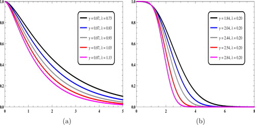
Figure 2. Diagrams displaying the PDF for different parametric values.

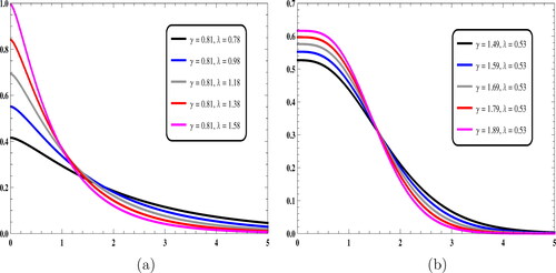
Figure 3. Three-dimensional mean and variance graphs for different parametric values.

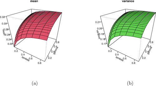
Figure 4. Skewness and kurtosis graphs in three dimensions for various parametric variables.

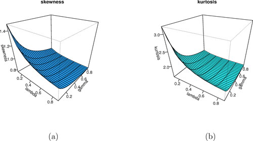
Figure 5. (a) $\beta$=1.0, $w=5.0$ and (b) $\beta$=1.5, $w=3.0$ RME plots for the EP model.

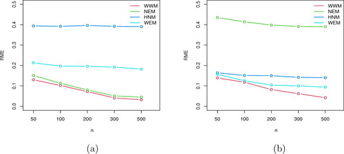
Table 1. For some parameter values, mean, variance, skewness, and kurtosis are present.

Parameters	$\gamma$ = 1
$\lambda$	Mean	Variance	Skewness	Kurtosis
2	0.5833	0.2847	1.7902	16.4277
4	0.2916	0.0711	1.7902	16.4277
6	0.1944	0.0316	1.7902	16.4277
8	0.1458	0.0177	1.7902	16.4277
10	0.1166	0.0113	1.7902	16.4277
12	0.0972	0.0079	1.7902	16.4277
Parameters	$\lambda$ = 2
$\gamma$	Mean	Variance	Skewness	Kurtosis
1	0.5833	0.2847	1.7902	16.4277
2	0.4628	0.1041	0.7808	28.7193
3	0.4556	0.0847	0.4451	38.4799
4	0.4585	0.0795	0.2869	44.1649
5	0.4625	0.0777	0.1999	47.5552
6	0.4663	0.0771	0.1470	49.6907

Table 2. When data from the EP model are simulated, RB and RME are used for the various estimations.

			Estimate
n	$\beta$	W	${\widehat{f}}_{\mathit{\text{ML}}}(0)$		${\widehat{f}}_{1,\mathit{\text{ML}}}(0)$		${\widehat{f}}_{2,\mathit{\text{ML}}}(0)$		${\widehat{f}}_{3,\mathit{\text{ML}}}(0)$
			RB	RME	RB	RME	RB	RME	RB	RME
50	1.0	5.0	−0.1751	0.1401	0.0520	0.1413	0.3751	0.3842	0.1825	0.2134
100	1.0	5.0	−0.1773	0.1101	0.0534	0.1132	0.3785	0.3822	0.1811	0.1972
200	1.0	5.0	−0.1794	0.0422	0.0437	0.0703	0.3847	0.3861	0.1804	0.1962
300	1.0	5.0	−0.1717	0.0413	0.0335	0.0416	0.3863	0.3828	0.1793	0.1920
500	1.0	5.0	−0.1757	0.0323	0.0231	0.0356	0.3843	0.3839	0.1678	0.1860
50	1.5	3.0	−0.1132	0.1291	0.4021	0.4355	0.1332	0.1640	0.0907	0.1578
100	1.5	3.0	−0.1172	0.1281	0.3872	0.4144	0.1378	0.1517	0.0872	0.1251
200	1.5	3.0	−0.1194	0.1261	0.3790	0.3782	0.1421	0.1506	0.0813	0.1046
300	1.5	3.0	−0.1112	0.1246	0.3661	0.3612	0.1325	0.1428	0.0801	0.1005
500	1.5	3.0	−0.1482	0.1317	0.3613	0.3501	0.1211	0.1406	0.0753	0.0241
50	2.0	2.5	−0.1001	0.1041	0.6016	0.6251	0.0232	0.1095	0.2451	0.2790
100	2.0	2.5	−0.1021	0.0632	0.5931	0.6080	0.0171	0.0782	0.2390	0.2601
200	2.0	2.5	−0.1104	0.0401	0.5752	0.5814	0.0052	0.0501	0.2253	0.2342
300	2.0	2.5	−0.1154	0.0210	0.5423	0.5565	0.0026	0.0401	0.2204	0.2123
500	2.0	2.5	−0.1196	0.0142	0.5351	0.5205	0.0013	0.0204	0.2125	0.2103
50	2.5	2.0	−0.0742	0.0746	0.7043	0.7241	0.1165	0.1527	0.3253	0.3512
100	2.5	2.0	−0.0786	0.0732	0.7975	0.7084	0.1288	0.1297	0.3202	0.3340
200	2.5	2.0	−0.0791	0.0712	0.7961	0.7024	0.1261	0.1183	0.3196	0.3272
300	2.5	2.0	−0.0843	0.0681	0.7920	0.7001	0.1220	0.1121	0.3153	0.3216
500	2.5	2.0	−0.0785	0.0630	0.7903	0.6929	0.1200	0.1090	0.3121	0.3173

Table 3. When data are simulating from the BE model, RB and RME for the various estimations.

			Estimate
n	$\beta$	W	${\widehat{f}}_{\mathit{\text{ML}}}(0)$		${\widehat{f}}_{1,\mathit{\text{ML}}}(0)$		${\widehat{f}}_{2,\mathit{\text{ML}}}(0)$		${\widehat{f}}_{3,\mathit{\text{ML}}}(0)$
			RB	RME	RB	RME	RB	RME	RB	RME
50	1.0	0.5	0.0601	0.0912	0.5094	0.5551	0.1913	0.2231	0.2844	0.2560
100	1.0	0.5	0.0521	0.0833	0.4882	0.5184	0.1890	0.2146	0.2431	0.2212
200	1.0	0.5	0.0341	0.0672	0.4710	0.5011	0.1825	0.1801	0.2003	0.2012
300	1.0	0.5	0.0280	0.0451	0.3962	0.5001	0.1732	0.1744	0.1901	0.1902
500	1.0	0.5	0.0092	0.0371	0.3612	0.4926	0.1384	0.1673	0.1801	0.1842
50	1.5	1.0	0.1724	0.1892	0.4110	0.4853	0.1791	0.2025	0.1682	0.2001
100	1.5	1.0	0.1532	0.1670	0.4322	0.4161	0.1472	0.1892	0.1361	0.1866
200	1.5	1.0	0.1413	0.1301	0.3236	0.3913	0.1386	0.1657	0.1172	0.1708
300	1.5	1.0	0.1061	0.1286	0.3202	0.3478	0.1291	0.1424	0.1163	0.1632
500	1.5	1.0	0.1001	0.1123	0.3172	0.3117	0.1031	0.1291	0.1012	0.1587
50	2.0	1.5	0.1251	0.1413	0.3991	0.4320	0.1985	0.2253	0.2101	0.1830
100	2.0	1.5	0.1074	0.1172	0.2846	0.3312	0.1626	0.2113	0.2061	0.1612
200	2.0	1.5	0.0665	0.0753	0.2312	0.2830	0.1357	0.1892	0.1946	0.1542
300	2.0	1.5	0.0517	0.0734	0.2196	0.2655	0.1224	0.1690	0.1912	0.1316
500	2.0	1.5	0.0473	0.0513	0.2167	0.2508	0.1115	0.1523	0.1820	0.1091
50	2.5	2.0	0.1410	0.1675	0.2513	0.3196	0.2498	0.2755	0.1994	0.2182
100	2.5	2.0	0.1302	0.1531	0.2432	0.2936	0.2001	0.2396	0.1701	0.1982
200	2.5	2.0	0.0921	0.1026	0.2312	0.2236	0.1927	0.2278	0.1583	0.1667
300	2.5	2.0	0.0802	0.1017	0.2272	0.2097	0.1812	0.2186	0.1423	0.1528
500	2.5	2.0	0.0801	0.0926	0.2213	0.2008	0.1723	0.2166	0.1382	0.1457

Table 4. Information regarding wooden stakes parallel distances in meters.

2.02	0.45	10.40	3.61	0.92	1.00	3.40	2.90	8.16	6.47	5.66
2.95	3.96	0.09	11.82	14.23	2.44	1.61	6.50	8.27	4.85	1.47
18.60	0.41	0.40	0.20	11.59	3.17	7.10	10.71	3.86	6.05	6.42
3.79	15.24	3.47	3.05	7.93	18.15	10.05	4.41	1.27	13.72	6.25
3.59	9.04	7.68	4.89	9.10	3.25	8.49	6.08	0.40	9.33	0.53
1.23	1.67	4.53	3.12	3.05	6.60	4.40	4.97	3.17	7.67	18.16
4.08

Figure 6. (c) $\beta$=2.0, $w=2.5$ and (d) $\beta$=2.5, $w=2.0$ RME plots for the EP model.

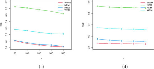
Figure 7. (a) $\beta$=1.0, $w=0.5$ and (b) $\beta$=1.5, $w=1.0$ RME plots for the BE model.

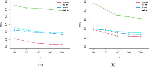
Figure 8. (c) $\beta$=2.0, $w=1.5$ and (d) $\beta$=2.5, $w=2.0$ RME plots for the BE model.

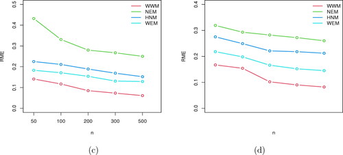
Figure 9. Box plot and TTT plot for wooden stakes dataset.

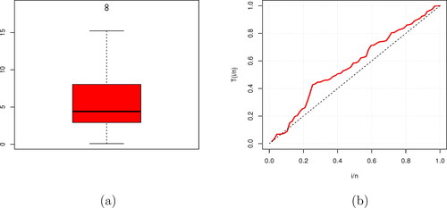
Table 5. The wooden stakes dataset’s descriptive statistics and related theoretical WWM metrics.

Sample size (n)	Mean	Median	Standard deviation	Skewness	Kurtosis	$\frac{\mathit{\text{Skewness}}}{\mathit{\text{Kurtosis}}}$
67	5.73201	4.41242	4.55640	1.10830	3.80333	0.29148
67	5.73370	4.47211	4.53042	1.31830	3.60312	0.36582

Table 6. The Hemmingway’s data perpendicular distance data in meters.

0	0	0	0	0	0	0	0	8.72	10.5
22.3	26.0	26.0	30.5	30.5	31.7	34.2	35.1	38.0	41.0
42.1	50.8	55.1	58.5	63.6	64.3	65.0	68.8	71.1	71.8
71.9	72.1	73.1	76.6	77.6	78.1	84.0	84.5	86.0	86.0
87.0	90.0	92.3	94.0	96.4	96.4	106.0	115.0	123.0	123.0
129.0	129.0	143.0	143.0	150.0	151.0	153.0	157.0	161.0	164.0
164.0	164.0	166.0	175.0	188.0	193.0	200.0	200.0	246.0	260.0
272.0	378.0	400.0

Figure 10. Box plot and TTT plot for Hemmingway’s dataset.

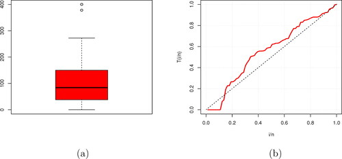
Table 7. Hemmingway’s dataset descriptive statistics and related theoretical WWM metrics.

Sample size (n)	Mean	Median	Standard deviation	Skewness	Kurtosis	$\frac{\mathit{\text{Skewness}}}{\mathit{\text{Kurtosis}}}$
73	99.2414	84.0012	82.3732	1.36056	5.47687	0.24841
73	99.9404	84.3516	82.3506	1.34128	4.83453	0.27742

Table 8. The MLEs, W*, A*, statistics K–S and p value for wooden stakes dataset.

Detection models	$\widehat{\gamma }$	$\widehat{\lambda }$	$A^{*}$	$W^{*}$	K–S	p Value
WWM	1.3756	0.0694	0.2471	0.0361	0.0819	0.7596
NDM	1.2845	0.1166	0.2641	0.2672	0.0840	0.7314
Model (2013)	2.1208	0.23506	0.2731	0.0385	0.0861	0.7019
GEM	1.7377	6.9115	0.2721	0.0420	0.0885	0.6705
EPSM	1.7377	9.4989	0.2721	0.0420	0.0885	0.6700
RLM	0.2838	6.7168	0.2596	0.0408	0.08907	0.6623
EQM	0.0072	0.0398	0.2792	0.0441	0.0909	0.6361
WHNM	–	42.698	0.8711	0.1512	0.1041	0.4610
Model (2015)	–	0.2369	0.3772	0.0702	0.1136	0.3520
WEM	–	0.2045	0.5024	0.0979	0.1261	0.2366
NEM	–	0.1747	1.0226	0.2065	0.1588	0.0680

Table 9. Information criteria and log-likelihood $(\mathcal{l})$ for wooden stakes dataset.

Detection models	−$\mathcal{l}$	AIC	AICC	BIC	HQIC	CAIC
WWM	181.703	367.008	367.195	371.017	369.053	367.095
NDM	181.662	367.325	367.512	371.734	369.069	367.512
Model (2013)	182.030	368.06	368.248	372.470	369.805	368.248
GEM	181.652	367.303	367.491	371.713	369.048	367.491
EPSM	181.652	367.303	367.491	371.713	369.048	367.491
RLM	181.768	367.536	367.723	371.945	369.281	367.723
EQM	181.656	367.311	367.499	371.720	369.056	367.499
WHNM	181.752	367.503	367.591	371.813	369.058	367.511
Model (2015)	182.165	367.330	367.392	371.535	369.203	367.392
WEM	182.526	367.052	367.213	371.156	369.924	367.113
NEM	183.862	369.723	369.785	371.928	370.596	369.785

Table 10. The MLEs, W*, A*, statistics K–S and p value for Hemmingway’s dataset.

Detection models	$\widehat{\gamma }$	$\widehat{\lambda }$	$A^{*}$	$W^{*}$	K–S	p Value
WWM	1.3181	0.0018	0.0120	0.0850	0.1095	0.3445
NDM	1.2265	0.0041	0.0864	0.0869	0.1095	0.3435
Model (2013)	1.5614	0.0125	0.0981	0.1014	0.1098	0.3131
GEM	1.3125	5.9110	0.0272	0.0420	0.1885	0.2708
EPSM	1.5905	15.965	0.1272	0.0969	0.1095	0.3444
RLM	6.0001	0.0160	0.2626	0.0886	0.1099	0.3440
EQM	0.0072	0.0398	0.2825	0.1068	0.1195	0.2498
WHNM	–	42.698	0.9167	0.1964	0.1223	0.2244
Model (2015)	–	0.0117	0.0772	0.0886	0.1156	0.3012
WEM	–	0.0117	0.0986	0.0886	0.1495	0.0912
NEM	–	0.0100	1.7216	0.2932	0.1443	0.0952

Table 11. Information criteria and log-likelihood $(\mathcal{l})$ for Hemmingway’s dataset.

Detection models	−$\mathcal{l}$	AIC	AICC	BIC	HQIC	CAIC
WWM	406.941	817.883	818.054	822.463	819.708	818.054
NDM	406.980	817.959	818.131	822.449	819.785	818.131
Model (2013)	407.572	819.145	819.316	823.725	820.970	819.316
GEM	407.501	818.303	819.491	822.713	819.748	818.491
EPSM	407.056	818.113	818.285	822.694	819.939	818.285
RLM	407.759	817.919	818.691	822.911	819.945	819.691
EQM	407.009	818.019	818.190	822.600	819.844	818.190
WHNM	408.842	819.685	819.741	822.975	820.598	819.741
Model (2015)	408.291	818.583	818.639	822.873	819.996	818.639
WEM	407.698	817.897	818.954	829.688	819.310	819.454
NEM	408.621	819.299	821.533	822.556	819.299	822.913

Table 12. For a wooden stake, the confidence intervals.

CI	$\gamma$	$\lambda$	$f(0)$
$95\%$	[0.2851, 2.4665]	[0, 1.1603]	[0, 1.2036]
$99\%$	[0, 2.8116]	[0, 1.5054]	[0, 1.5487]

Table 13. For Hemmingway’s dataset, the confidence intervals.

CI	$\gamma$	$\lambda$	$f(0)$
$95\%$	[0, 20.214]	[0, 18.898]	[0, 18.903]
$99\%$	[0, 26.152]	[0, 24.836]	[0, 24.827]

Table 14. Estimated population abundance D and $f(0;\lambda ,\gamma )$ for the wooden stakes dataset using the $|\widehat{\mathit{\text{SD}}}-\mathit{\text{SD}}|.$

Detection models	${\widehat{f}}_{\mathit{\text{ML}}}(0)$	$(\widehat{D})$	$|\widehat{\mathit{\text{SD}}}-\mathit{\text{SD}}|$
WWM	0.11271	0.00370	0.02603
NDM	0.11402	0.00384	0.02907
Model (2013)	0.09504	0.00322	0.26611
GEM	0.11820	0.00393	0.03210
EPSM	0.11804	0.00397	0.03206
RLM	0.12006	0.00401	0.03640
EQM	0.12202	0.00401	0.03410
WHNM	0.09401	0.00320	0.33963
Model (2015)	0.12911	0.00430	0.41671
WEM	0.13600	0.00457	0.66913
NEM	0.17401	0.00580	1.17652

Table 15. Estimated population abundance D and $f(0;\lambda ,\gamma )$ for the Hemmingway’s dataset using the $|\widehat{\mathit{\text{SD}}}-\mathit{\text{SD}}|.$

Detection models	${\widehat{f}}_{\mathit{\text{ML}}}(0)$	$(\widehat{D})$	$|\widehat{\mathit{\text{SD}}}-\mathit{\text{SD}}|$
WWM	0.00659	0.00024	0.02201
NDM	0.00657	0.00024	0.02906
Model (2013)	0.00656	0.00023	0.26911
GEM	0.11820	0.00393	0.03120
EPSM	0.00710	0.00025	0.03761
RLM	0.00700	0.00025	0.03649
EQM	0.00764	0.00027	0.03643
WHNM	0.00530	0.00019	0.32190
Model (2015)	0.02550	0.00090	0.31672
WEM	0.00781	0.00028	0.64321
NEM	0.01007	0.00036	1.18136