Creating optimized machine learning pipelines for PV power generation forecasting using the grid search and tree-based pipeline optimization tool

Figures & data

Figure 1. Machine learning pipeline structure.

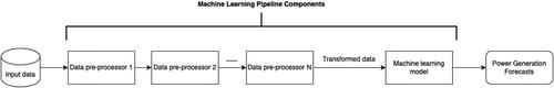
Figure 2. An example of scheduling the appliances’ working hours in the farm, based on the power generation forecasts given by the created optimal ML pipeline.

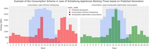
Figure 3. Main components of the farm’s solar power system.

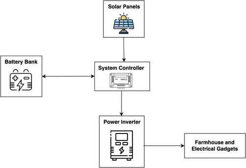
Figure 4. Training process visualization.

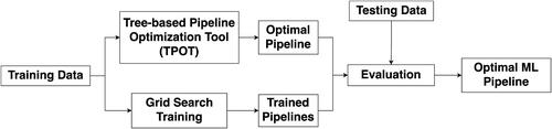
Figure 5. Dataset splitting strategy for the training and testing processes.

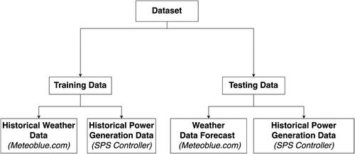
Figure 6. The experimental setup.

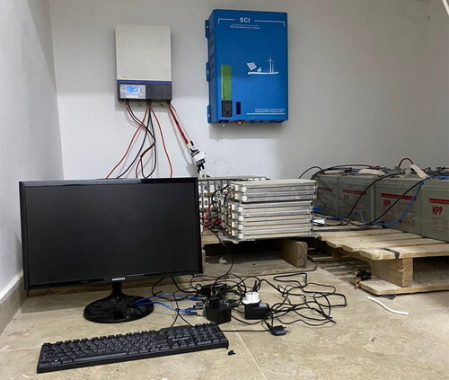
Table 1. Sample of raw data exported from the SPS controller.

Month	Day	Hour	Minutes	PV Voltage (Volt)	PV Power (Watt)	Output voltage (Volt)	Load (Watt)	Frequency (Hz)	Load (%)	Battery (%)
2	9	5	38	233	116	227	4065	50	92	17
2	9	5	38	235	119	227	4068	50	92	16
2	9	5	38	235	119	227	4068	50	92	16
2	9	5	40	243	119	229	3177	50	72	15
2	9	6	00	221	685	230	3682	50	74	100

Figure 7. Correlation Matrix: Features Pearson Correlation.

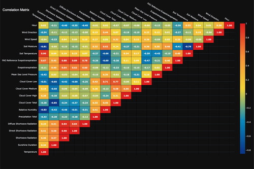
Figure 8. Visualization of Adaboost working procedure given a sample of data points. (Raschka et al. 2022a).

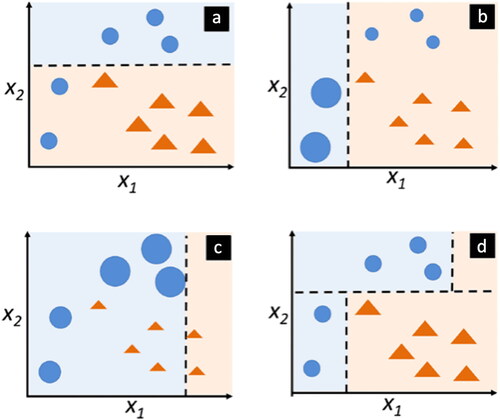
Table 2. Grid Search involved regressors, tuned hyperparameters, and the number of trained regressors and total pipelines.

Model’s algorithm	Tuned hyperparameters	Number of models trained	Number of pipelines
Support Vector Machine (SVM)	Kernal, C, epsilon, gamma	120	360
Lasso Regression	Lasso_alphas, selection	42	126
Ridge Regression	Alpha, solver	105	315
Adaboost Regressor	Loss, learning_rate, n_estimators	60	180
Gradient Boosting Regressor	Loss, learning_rate, n_estimators, max_depth, min_samples_split, min_samples_leaf	1920	5760
XGBoost Regressor	Booster, tree_method, n_estimators, learning_rate, min_split_loss, max_depth, reg_lambda, reg_alpha	720	2160
Random Forests Regressor	n_estimators, max_features, max_depth, min_samples_split, min_samples_leaf, bootstrap	480	1440

Figure 9. Machine learning pipeline steps automated by TPOT.

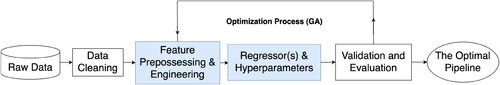
Figure 10. NMAE values distribution, grouped by each hour.

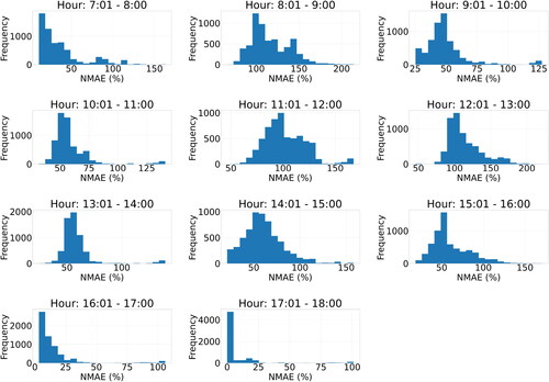
Figure 11. ANMAE values distribution for all the experimented pipelines.

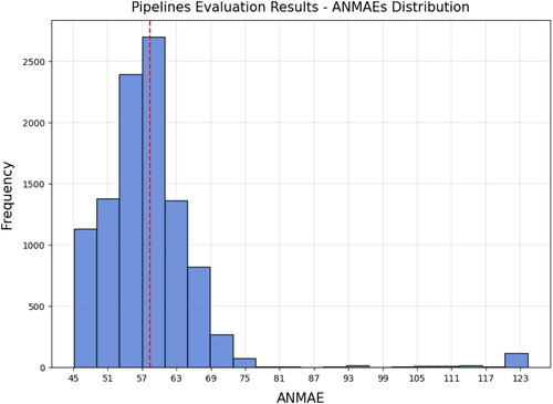
Figure 12. PRMSE values distribution for all the experimented pipelines.

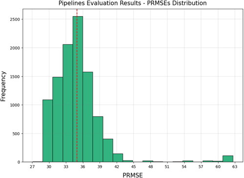
Table 3. Details of top and bottom 3 pipelines resulted from the 2 optimization methods: Grid Search and TPOT.

Pipeline rank	Preprocessor	Regressor	Regressor hyperparameters	Optimization method	ANMAE (%)	PRMSE (%)
1st	Power Transformer	Gradient Boosting Regressor	{’loss’: ’absolute_error’, ’learning_rate’: 0.1, ’max_depth’: 25, ’n_estimators’: 1250, ’min_samples_leaf’: 1, ’min_samples_split’: 7}	GS	46.31	27.07
2nd	Power Transformer	Gradient Boosting Regressor	{’loss’: ’absolute_error’, ’learning_rate’: 0.1, ’max_depth’: 13, ’n_estimators’: 200, ’min_samples_leaf’: 1, ’min_samples_split’: 7}	GS	46.61	29.11
3rd	Power Transformer	Gradient Boosting Regressor	{’loss’: ’absolute_error’, ’learning_rate’: 0.1, ’max_depth’: 13, ’n_estimators’: 1750, ’min_samples_leaf’: 1, ’min_samples_split’: 5}	GS	46.81	29.43
6251st	Null	SVR	{’kernel’: ’rbf’, ’C’: 1, epsilon’: 3, ’gamma’: ’auto’}	GS	126.30	60.13
6252nd	Null	SVR	{’kernel’: ’rbf’, ’C’: 0.1, ’epsilon’: 3, ’gamma’: ’auto’}	GS	126.31	60.87
6253rd	Null	SVR	{’kernel’: ’sigmoid’, ’C’: 0.1, ’epsilon’: 0.5, ’gamma’: ’auto’}	GS	126.32	62.6

Figure 13. Lowest ANMAE achieved by each regressor type.

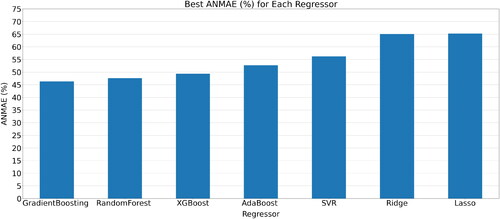
Figure 14. ANMAE achieved by the best pipeline resulted from each of the 2 optimization methods.

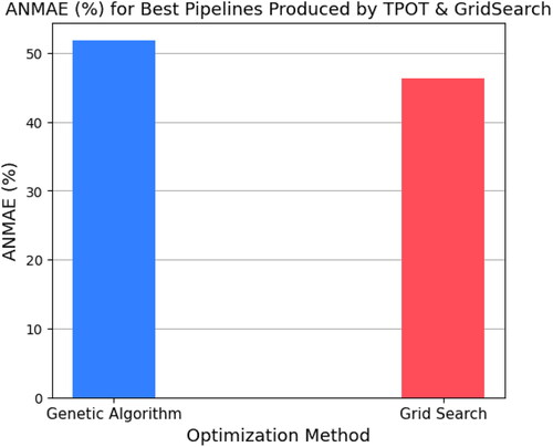
Table 4. Details of best pipeline resulted from each of the 2 optimization methods: Grid Search and TPOT.

Preprocessor(s)	Regressor	Regressor tunned hyperparameters	Optimization method	ANMAE (%)	PRMSE (%)
Power Transformer	Gradient Boosting Regressor	{’loss’: ’absolute_error’, ’learning_rate’: 0.1, ’max_depth’: 25, ’n_estimators’: 1250, ’min_samples_leaf’: 1, ’min_samples_split’: 7}	GS	46.31	27.07%
MaxNormalizer  + MaxAbsoluteScaler	StackingEstimator (RandomForest  + GradientBoost)	1. RandomForest: {max_features: 0.5, min_samples_leaf: 5, min_samples_split: 3} 2. GradientBoosting: {alpha: 0.95, max_depth: 10, max_features: 0.3, min_samples_leaf: 16, min_samples_split: 4}	GA (TPOT)	51.81	30.16%

Raschka, S., Liu, Y., Mirjalili, V., & Dzhulgakov, D. (2022a). Leveraging weak learners via adaptive boosting. Packt Publishing.

 Google Scholar

Data availability statement

Data are available on request from the authors.