Performance evaluation and CFD investigation of scraped surface ice cream freezer augmented with LN₂ freezing technique

Figures & data

Figure 1. Process and flow diagram for the connections made in SSF.

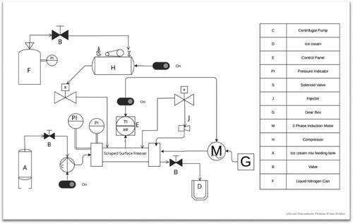
Figure 2. Isometric view, front view, and side view of the blade and rotor assembly.

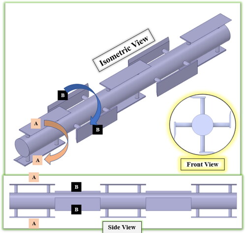
Table 1. Independent variables selected for optimization process for ice cream mixture as feed.

Process parameters (factors)	Values
A: Feed flow rate	200 to 240 lit/hr
B: Scraper speed	125 rpm (kept constant)
C: Liquid nitrogen temperature	−95 to −75 ˚C

Figure 3. Geometry of SSF.

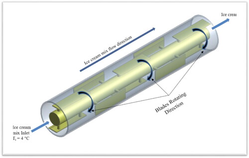
Table 2. Geometrical characteristics of SSF.

Geometrical parameters	Symbol	Value
Length of the heat transfer tube	L	0.7 m
Inside diameter of the heat transfer tube	Dt	0.12 m
Outside diameter of the heat transfer tube	Do	0.128 m
Thickness of the heat transfer tube	t	0.004 m
Rotor or shaft diameter	Ds	0.05 m
Inside jacket diameter	Dj	0.168 m
Outside jacket diameter	Dj2	0.180 m

Figure 4. Model fitted curve for the variation of (a) specific heat, (b) density, (c) thermal conductivity, and (c) viscosity with static temperature obtained in ANSYS Fluent.

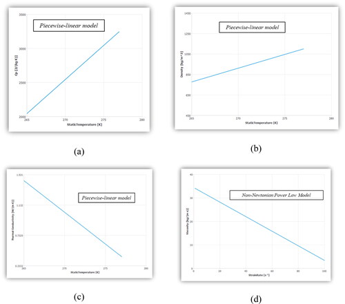
Table 3. Thermal properties of LN₂ obtained from fluent database.

Density [kg/m^3]	Specific heat [J/(kg K)]	Thermal conductivity [W/(mK)]	Viscosity [kg/(ms)]
806.08	2041.5	0.14581	0.00016065

Table 4. Thermal properties of solid material (steel) applied from the fluent database.

Density [kg/m^3]	Specific heat [J/(kg K)]	Thermal conductivity [W/(mK)]
8030	502.48	16.27

Figure 5. Tetrahedral meshing of (a) blade and rotor assembly (b) around the surface of heat transfer tube and the jacket.

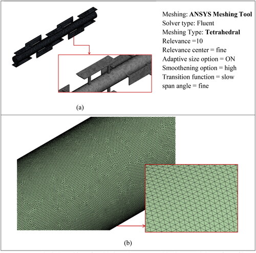
Figure 6. The relationship between ice cream output temperature and mesh element size variation.

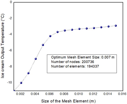
Figure 7. Effect of feed flow rate and LN₂ temperature on the (a) drawing temperature and (b) overall heat transfer coefficient at scraper speed of 125 rpm.

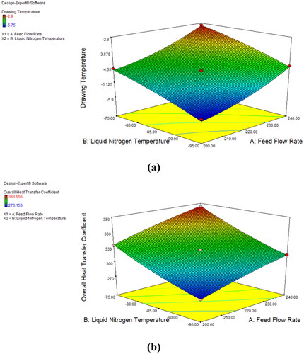
Figure 8. Scatter plot illustrating the relationship between internally studentized residuals and Predicted values for the (a) drawing temperature and (b) overall heat transfer coefficient as the response variables.

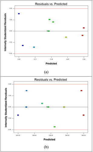
Figure 9. CFD parametric results obtained for the (a) output temperature condition, (b) velocity, and (c) pressure drop with varying feed flow rate and scraper speed.

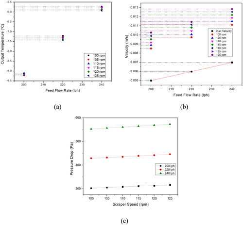
Figure 10. Velocity field in SSF obtained under reference operating conditions as predicted by numerical modeling.

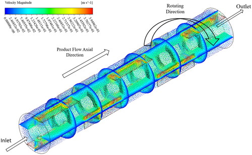
Figure 11. Velocity profile distribution under reference operating conditions V̇_mix = 240 lph, T_R = −95 °C, and N_rotor =125 rpm in the sectional plane A–A (right side) and B–B (left side).

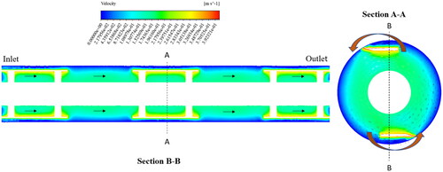
Figure 12. Temperature profile distribution under reference operating conditions V̇_mix = 240 lph, T_R = -95 °C, and N_rotor =125 rpm in the sectional plane A–A (right side) and B–B (left side).

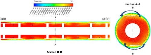
Figure 13. Pressure distribution under reference operating conditions V̇_mix = 240 lph, T_R = −95 °C, and N_rotor =125 rpm in the sectional plane A–A (right side) and B–B (left side).

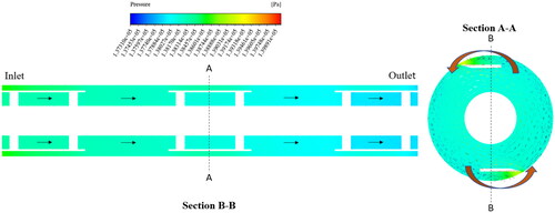
Figure 14. Temperature variation along axial distance of SSF for reference operating conditions V̇_mix = 240 lph, T_R = −95 °C, and N_rotor =125 rpm.

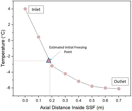
Figure 15. Comparison of experimental and CFD results of ice cream exit temperature under reference operating conditions.

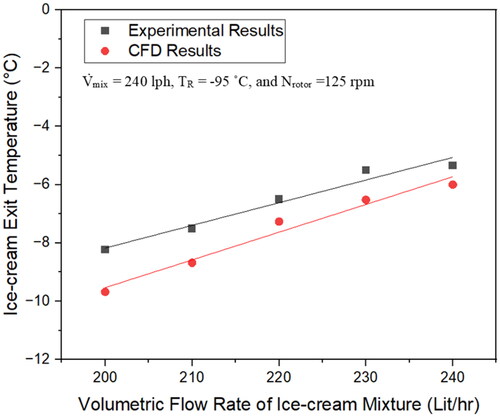
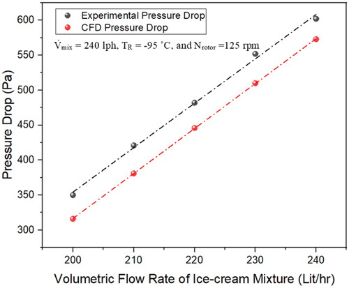
Figure 16. Comparison of experimental and CFD pressure drop results while passing the ice cream mixture through SSF under reference operating conditions.

Data availability statement

All data used for this research is included in this manuscript.