Modelling the impact of agrometeorological variables on regional tea yield variability in South Indian tea-growing regions: 1981-2015

Figures & data

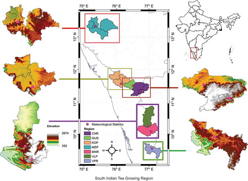
Figure 1. Map of elevation range and meteorological stations in the SITR. Black lines with the cross line are the boundary of tea growing region, grey lines are administrative boundaries of districts and blue line are state boundaries of India. The base map of India including administrative units at different levels was acquired in vector format with data available from GADM database of Global Administrative Areas (http://gadn.org/country) and processed using ESRI® ArcMap Version 10.1.

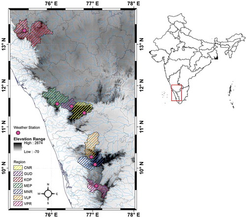
Table 1. Location of weather stations and data summary of the tea growing districts of South India

Locations	Code	Lat	Log	MSL	YPH	Tmax	Tmin	RH830	RH1430	RF	Rday	S	Sday	W	S830	S1430	Sm	ETo	Cloud
Coonoor	CNR	76.80	11.34	1790	2114	22.2	13.8	78	75	1777	89	6.17	323	1.59	18.1	18.2	0.76	100	2.04
Gudalur	GUD	76.49	11.50	815	2667	27.0	14.5	87	72	2173	116	8.32	272	1.89	12.8	12.9	0.80	106	1.82
Koppa	KOP	75.36	13.53	630	2699	29.7	20.2	85	67	2186	130	7.32	284	1.80	27.9	28.0	0.76	119	2.11
Meppadi	MEP	76.14	11.56	815	2146	28.6	18.4	91	72	2843	135	8.27	342	1.96	26.3	26.4	0.82	120	2.04
Munnar	MUN	77.06	10.09	1467	2077	22.3	12.7	91	77	4051	149	5.22	274	2.08	9.4	9.5	0.85	88	2.30
Valparai	VLP	76.97	10.27	1064	2417	25.8	15.9	88	74	3822	160	6.05	290	1.30	15.1	15.3	0.82	97	2.19
Vandiperiyar	VPR	77.09	9.57	860	1874	27.1	18.1	91	72	1825	131	5.00	269	1.90	16.6	16.7	0.81	95	2.09

Values are annual means of meteorological variables and total yield calculated across all years for each location. MSL: Mean above sea level (m); YPH: yield per hector (kg ha⁻¹); Tmin: temperature minimum (°C); Tmax: temperature maximum (°C); RH830h; relative humidity at 830 h (%); RH1430h: relative humidity at 1430 h (%); RF: Annual total rainfall (mm); Rday: mean number of rain day in a year (if $>$0.20 mm day⁻¹); S: sunshine hour (h); Sday: mean number of sunny days in a year (if $>$0.10 h day⁻¹); W: wind speed (km day⁻¹); S830: minimum soil temperature (°C); S1430: maximum soil temperature (°C); Sm: Soil moisture (%); ETo: evapotranspiration (mm); and Cloud: cloudiness (%).

Figure 2. Crop variability in terms of coefficient of variation (CV%) and standard deviation (STD) for monthly (a), seasonal (b) and annual tea yield (c) over SITR for 1981–2015. The horizontal line in the boxes indicates mean (thick) and median (thin) tea yield (kg ha⁻¹), the lower boundary of the box indicates the standard deviation (STD) while the upper boundary of the box indicates 95% percentiles. The lower and upper whiskers representing the minimum and maximum observed value. Filled circles at both below and above the whiskers indicate outliers. Values at the bottom represent the percentage of coefficient of variation (CV) is the ratio of the standard deviation to the mean.

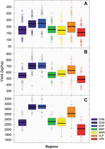
Table 2. Coefficient of multiple linear regression

Region	Tmin	Tmax	RH830	RH1430	RF	Rday	S	Sday	W	S830	S1430	Sm	ETo	Cloud	${\mathbf{R}}^{\mathbf{2}}$
Month
CNR	37.9***	−18.5***	5.78	7.05	0.36	1.13	−0.04	2.47**	−645.9	945.7***	−959.1***	175.6***	−0.40	−52.1***	0.438
GUD	0.99	1.49	6.97	7.41	0.30	−0.73	−12.9	2.78	−626.4	75.94	−73.59	−14.12	−0.38*	5.70	0.398
KOP	21.4***	−21.6***	9.52	9.53	0.40	−0.20	8.57*	1.19	−719.0	−366.2	369.3	−42.88	0.45	−59.6***	0.448
MEP	7.44***	−11.3***	−3.81	−2.35	−0.28	0.17	−6.06	1.84	447.2	26.24	−25.89	−369.2	−0.03	−30.5***	0.156
MNR	10.8***	6.86*	5.99	7.95	0.36	−1.22	−3.48	−0.96	−691.0	−326.0**	330.9**	128.6	0.32	−5.61	0.365
VLP	6.01***	30.4***	31.00***	2.44***	−0.02*	−1.35*	−13.3***	0.24	−2703***	−571.5*	563.5*	68.03	0.64	−20.1***	0.542
VPR	17.3***	−6.62**	−4.73	−5.05	−0.30	−0.20	0.98	1.46**	507.6	−169.6	170.1	−148.8	−0.21	−14.5**	0.389
Season
CNR	72.3**	−61.2**	−5.15	−7.19	−0.18	1.55	−23.8	1.30	653.8	1577.9*	−1596.3*	480.9*	1.30	−147.1**	0.295
GUD	0.83	5.85	−18.7	−17.9	−0.44	−0.57	−120.9*	8.23**	1663.6	165.03	−162.16	−20.46	−0.90	31.02	0.136
KOP	15.6	−24.9	13.8	10.7	0.17	2.57*	63.9**	0.78	−845.9	−1664.5	1678.5	−294.5	−0.76	−51.10	0.318
MEP	−38.8***	10.8*	−5.03	−6.75	0.00	0.76	1.40	0.48	134.7	−935.10	935.80	801.6	−84.53***	1.93	0.123
MNR	5.30	3.80	4.65	11.8	−0.07	1.04	−19.3	−0.11	617.0	−2106.0***	2129.0***	−3593.0	3.41	−22.87	0.319
VLP	−11.1	68.2**	55.4***	5.81*	−0.01	−0.40	−0.36	−0.60	−4330.0***	−242.90	237.40	−241.5	−1.90	−9.547	0.286
VPR	21.0*	−28.1*	4.89	5.06	−0.05	0.34	−17.0	1.26	−282.7	1328.0	−1311.0	370.0	2.75	−12.44	0.287
Annual
CNR	223.2	−473.8	−8.40	−115.5	−0.17	6.09	−566.6	4.86	6583	−15,150*	15,280*	1096	81.5	−916.6*	0.344
GUD	72.33	9.585	6.39	7.956	0.29	−0.84	1807.9*	−34.0*	−1058	−1028	963.2	−489.4	−6.92	54.43	0.031
KOP	89.61	−641.8	−6.30	−25.38	0.39	1.55	323.7	2.13	2178	3309	−2787	−2677	−21.3	−893.4	0.612
MEP	41.98	−69.16	79.2	109.5	−0.54	2.77	314.5	5.10	15,260	−5100	5035	−56,820*	−4.82	−25.44	0.392
MNR	126.4	69.79	−67.3	−73.18	0.60	4.77	−87.0	1.67	−12,640	−19,570	19,660	32,870	13.22	−457.8	0.480
VLP	−234.5	913.4*	194.9	65.81	−0.10	0.01	1528.0*	−5.68	−18,800*	9097	−8958	−7103	−247.0*	−191.7	0.550
VPR	311.2	−195.3	−10.0	−6.696	−0.45	7.35*	−162.0	5.61*	−885	6097	−6236	7649	21.0	−38.42	0.317

$R^2$: Regression coefficient; RMSE: Root means squared error; MAPE: mean absolute percentage error; $r$: correlation coefficient; All other designations are the same as those in the footnotes below Table 1.

Table 3. Predictive performance of statistical models during calibration and testing periods for the crop yield of SITR

Region	Month							Season							Annual
	${\mathbf{R}}^{\mathbf{2}}$	Calibration Period			Testing period			${\mathbf{R}}^{\mathbf{2}}$	Calibration Period			Testing period			${\mathbf{R}}^{\mathbf{2}}$	Calibration Period			Testing period
		RMSE	MAPE	r	RMSE	MAPE	r		RMSE	MAPE	r	RMSE	MAPE	r		RMSE	MAPE	r	RMSE	MAPE	r
SMLR
CNR	0.452	33.7	15.0	0.67	33.1	16.1	0.67	0.233	68.1	9.87	0.47	49.7	7.06	0.64	0.227	172.0	5.98	0.58	38.8	1.14	0.13
GUD	0.028	36.8	13.0	0.13	32.9	12.8	0.52	0.103	80.5	9.08	0.10	52.8	6.34	0.09	0.327	147.4	4.36	0.26	137.5	3.75	0.69
KOP	0.473	34.9	12.9	0.65	35.0	11.8	0.75	0.357	67.9	7.94	0.01	51.5	5.59	0.24	0.785	60.8	1.82	0.60	118.6	3.15	0.95
MEP	0.175	33.4	15.0	0.41	40.8	18.7	0.50	0.067	65.1	9.30	0.22	64.3	9.14	0.37	0.483	136.6	4.51	0.77	80.7	2.81	0.29
MNR	0.382	37.6	17.4	0.65	50.3	24.1	0.46	0.377	70.3	10.2	0.28	78.9	9.00	0.06	0.570	190.0	7.51	0.20	69.0	2.64	0.46
VLP	0.556	36.7	14.7	0.79	50.1	25.3	0.41	0.346	90.6	11.5	0.34	71.0	9.36	0.14	0.401	271.0	8.25	0.30	260.1	7.59	0.00
VPR	0.398	30.4	17.3	0.67	42.2	20.3	0.46	0.347	61.8	10.9	0.41	70.5	10.8	0.21	0.382	204.6	8.94	0.51	112.4	4.86	0.57
ARIMAX
CNR	0.640	28.5	12.6	0.78	23.3	10.9	0.86	0.700	59.7	8.67	0.63	47.1	6.69	0.65	0.790	137.2	4.83	0.15	71.6	2.79	0.38
GUD	0.700	24.9	9.2	0.75	27.8	10.5	0.63	0.490	60.3	6.43	0.11	41.6	4.65	0.25	0.740	160.6	4.38	0.11	107.1	3.46	0.23
KOP	0.710	34.5	12.6	0.68	31.9	10.5	0.79	0.620	69.1	8.24	0.13	49.8	4.97	0.20	0.680	165.7	4.06	0.53	120.9	2.70	0.67
MEP	0.700	27.2	12.0	0.70	31.1	13.8	0.73	0.860	52.1	7.37	0.20	52.9	7.70	0.07	0.690	100.3	3.58	0.98	74.5	2.69	0.62
MNR	0.850	31.1	14.4	0.78	35.8	14.2	0.75	0.910	48.1	7.22	0.34	62.7	8.00	0.02	0.770	126.8	4.62	0.32	89.5	2.66	0.98
VLP	0.810	33.8	13.5	0.83	31.4	13.2	0.79	0.920	67.3	8.95	0.36	70.8	9.30	0.35	0.820	145.0	4.32	0.82	149.7	4.36	0.25
VPR	0.600	25.5	13.0	0.79	26.1	12.1	0.83	0.770	218.2	30.5	0.28	192.0	27.5	0.20	0.790	361.8	16.20	0.47	236.8	9.39	0.42
ANN
CNR	0.916	17.9	6.79	0.93	24.0	9.18	0.86	0.794	63.2	8.67	0.64	62.6	9.01	0.43	0.642	73.4	2.22	0.83	120.9	3.08	0.98
GUD	0.864	20.1	4.34	0.86	15.7	3.23	0.90	0.800	50.4	3.47	0.12	20.1	1.96	0.47	0.524	189.0	3.12	0.82	60.5	1.42	0.73
KOP	0.912	20.7	5.17	0.90	21.6	5.16	0.93	0.857	41.7	2.52	0.09	19.0	0.92	0.25	0.830	92.7	2.26	0.90	79.9	1.58	0.13
MEP	0.863	19.7	5.54	0.86	23.0	5.68	0.89	0.846	46.3	3.77	0.24	30.8	3.01	0.50	0.887	101.8	2.00	0.71	31.5	0.73	0.25
MNR	0.918	18.8	6.74	0.92	26.8	7.55	0.90	0.914	37.3	3.13	0.32	21.3	1.85	0.36	0.919	85.6	2.96	0.90	163.2	3.53	0.66
VLP	0.921	24.6	6.40	0.92	19.4	5.37	0.93	0.850	53.8	5.22	0.24	70.4	6.38	0.26	0.931	113.4	3.43	0.90	51.5	1.65	0.86
VPR	0.899	20.6	7.98	0.90	20.4	7.36	0.90	0.901	34.7	3.99	0.39	22.7	3.62	0.50	0.893	142.9	3.53	0.86	58.9	1.78	0.88
VAR
CNR	0.729	21.0	9.52	0.85	19.1	8.52	0.88	0.505	42.3	6.09	0.71	35.6	5.04	0.70	0.727	107.3	3.80	0.72	86.3	3.31	0.39
GUD	0.638	21.4	7.89	0.80	21.7	8.17	0.76	0.626	48.4	5.20	0.12	42.5	4.71	0.21	0.668	108.1	2.56	0.80	85.6	2.39	0.72
KOP	0.745	21.8	7.83	0.85	24.4	8.34	0.88	0.716	23.2	2.69	0.26	21.9	2.53	0.35	0.950	76.4	1.86	0.90	59.6	1.58	0.89
MEP	0.649	23.2	10.6	0.80	26.1	11.6	0.83	0.499	45.2	6.40	0.26	38.8	5.83	0.55	0.935	57.5	1.91	0.20	44.4	1.59	0.48
MNR	0.574	21.9	10.6	0.75	24.5	9.18	0.79	0.658	50.5	7.35	0.27	56.0	7.38	0.05	0.865	98.5	3.83	0.08	57.2	1.96	0.93
VLP	0.700	24.6	9.58	0.84	25.2	10.6	0.82	0.763	41.0	5.33	0.24	41.6	5.40	0.30	0.897	105.4	3.15	0.79	87.4	3.05	0.57
VPR	0.711	19.5	10.4	0.85	22.1	10.3	0.84	0.724	37.1	6.02	0.40	54.5	8.22	0.57	0.934	68.1	2.44	0.89	52.9	2.06	0.74

R²: Regression coefficient; RMSE: Root means squared error; MAPE: mean absolute percentage error; r: correlation coefficient; All other designations are the same as those in the footnotes below Table 1.

Figure 3. Comparison of observed and modelled monthly tea yield (kg/ha; y axis) of Valparai during calibration (a) and testing period (b), and cross-validation plot at various temporal scales (c). Observed yield (kg/ha) in the x-axis (in the top and in the bottom) and predicted yield (kg/ha) y-axis (in the left and right). OBS: observed tea yield; and modelled yield by SMLR: step-wise multiple linear regression; SARIMAX: Seasonal autoregressive integrated moving average; ANN: artificial neural network; and VAR: Vector autoregressive model.

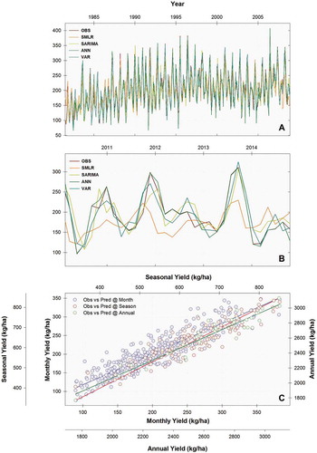
Figure 4. Box Plot of observed and modelled tea yield over SITR. Left, centre and right panel shows monthly (a-g), seasonal (h-n) and annual (o-u) tea yield, respectively. The regional codes are the same as those in the footnotes below Figure 2, but for model performance.

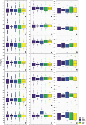
Figure 5. Impulse response functions of climate variables on tea yield (y-axis), Response of YPH (a & e), Tmin (b & f), Tmax (c & g) and RF (d & h) at seasonal (a-d) and annual (e-h) time series.

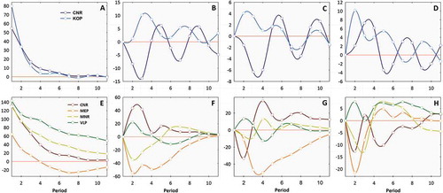
Table 4. Granger causality test

Month	CNR	GUD	KOP	MEP	MNR	VLP	VPR
Tmax	16.8***	4.62***	3.14***	5.31***	4.44***	5.49***	8.65***
Tmin	14.4***	2.85**	1.84**	6.76***	4.36***	12.6***	14.4***
RH830	7.06***	0.32^ns	0.73^ns	3.43***	2.95**	2.28**	5.07***
RH1430	11.9***	0.31^ns	1.19^ns	2.54**	3.48***	9.75***	5.14***
RF	6.53***	2.10*	2.17**	6.97***	5.73***	9.46***	10.8***
Rday	11.8***	1.50^ns	2.53***	6.84***	5.25***	10.4***	9.75***
S	8.67***	1.96*	4.56***	6.71***	9.62***	9.88***	6.31***
Sday	4.65***	2.33**	2.06**	8.36***	6.19***	10.2***	7.12***
W	10.4***	1.14^ns	1.45^ns	5.99***	4.81***	1.75^ns	8.83***
S830	19.6***	2.65**	3.06***	6.77***	7.19***	10.7***	3.09***
S1430	19.6***	2.66**	3.09***	6.76***	7.20***	10.7***	3.02**
Sm	6.88***	0.70^ns	1.25^ns	3.80***	3.39***	7.87***	5.83***
ETo	15.4***	1.75^ns	3.16***	7.33***	8.85***	10.2***	4.95***
Cloud	7.47***	0.61^ns	1.75*	5.57***	5.04***	7.29***	8.04***
Season
Tmax	6.15***	0.30^ns	2.63*	0.81^ns	1.52^ns	4.98***	16.9***
Tmin	5.96***	0.43^ns	2.87*	3.47**	1.88^ns	4.17***	14.8***
RH830	2.74**	0.25^ns	1.65^ns	1.41^ns	5.94**	2.70**	4.45**
RH1430	3.06***	0.48^ns	6.36***	2.76*	2.09^ns	6.19***	29.2***
RF	2.94**	0.18^ns	3.62**	4.97***	1.88^ns	4.24***	27.0***
Rday	3.67***	0.33^ns	4.54**	5.40***	1.79^ns	6.24***	21.8***
S	4.65***	0.21^ns	5.79***	5.38***	1.31^ns	5.94***	27.0***
Sday	3.26**	0.29^ns	3.99**	4.68**	1.77^ns	4.51***	18.5***
W	3.12**	0.32^ns	5.04***	4.15**	2.19^ns	2.18*	32.3***
S830	6.72***	1.00^ns	3.81**	4.15**	0.68^ns	3.56***	12.6***
S1430	6.72***	1.01^ns	3.78**	4.15**	0.70^ns	3.57***	13.0***
Sm	3.50***	0.27^ns	6.16***	2.72*	2.73*	5.59***	7.42***
ETo	4.50***	0.25^ns	4.82**	2.63*	1.53^ns	4.78***	19.5***
Cloud	3.46**	0.35^ns	4.67**	2.19^ns	1.78^ns	4.90***	37.5***
Annual
Tmax	1.77^ns	1.80^ns	0.25^ns	4.68**	0.30^ns	0.00^ns	0.67^ns
Tmin	0.17^ns	1.51^ns	0.40^ns	0.86^ns	0.04^ns	0.29^ns	0.33^ns
RH830	0.26^ns	0.12^ns	0.20^ns	1.64^ns	0.61^ns	0.18^ns	0.55^ns
RH1430	0.04^ns	0.30^ns	3.56*	0.73^ns	0.34^ns	3.57*	0.35^ns
RF	0.60^ns	0.15^ns	3.47*	0.71^ns	0.02^ns	0.27^ns	1.01^ns
Rday	0.10^ns	0.00^ns	0.90^ns	0.01^ns	0.03^ns	0.00^ns	14.3
S	1.32^ns	0.01^ns	5.32**	0.15^ns	0.26^ns	2.37^ns	0.87^ns
Sday	0.11^ns	0.03^ns	1.36^ns	0.39^ns	0.11^ns	0.09^ns	2.71^ns
W	0.09^ns	0.01^ns	0.30^ns	1.51^ns	0.56^ns	0.75^ns	0.26^ns
S830	0.55^ns	1.83^ns	0.20^ns	3.56*	0.27^ns	0.41^ns	0.81^ns
S1430	0.52^ns	1.92^ns	0.20^ns	3.55*	0.26^ns	0.42^ns	0.83^ns
Sm	0.06^ns	0.44^ns	0.01^ns	1.14^ns	0.64^ns	4.18**	1.10^ns
ETo	0.52^ns	0.43^ns	2.53^ns	1.01^ns	1.43^ns	1.22^ns	1.83^ns
Cloud	0.50^ns	0.30^ns	0.88^ns	3.10*	0.15^ns	0.22^ns	0.28^ns

All designations are the same as those in the footnotes below Table 1.

Figure 6. First order (FS: in Orange) and total global sensitivity (GS: in Red) of tea yield (kg ha⁻¹) due to climate variability at month (a-g, top panel), season (h-o, middle panel) and annual (P-V, bottom panel) scales. All abbreviations are the same as those in the footnotes below Table 1.

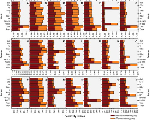
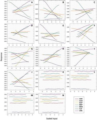
Figure 7. Region and variable specific global sensitivity response at month, season and annual tea productivity. (a): Tmin (°C); (b): Tmax (°C); (c): RH830h (%); (d): RH1430h (%); (e): RF (mm); (f): Rday; (g): S (h); (h): Sday; (i): W (k day⁻¹); (j): S830 (°C); (k): S1430h (°C); (l): Sm (%); (m): ETo (mm); (n): Cloud (%).