Figures & data
Figure 1. Autocorrelation plot of eggs consumption data used to test for stationarity.
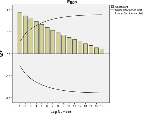
Figure 2. ACF plot after first-order differencing of the eggs consumption data.
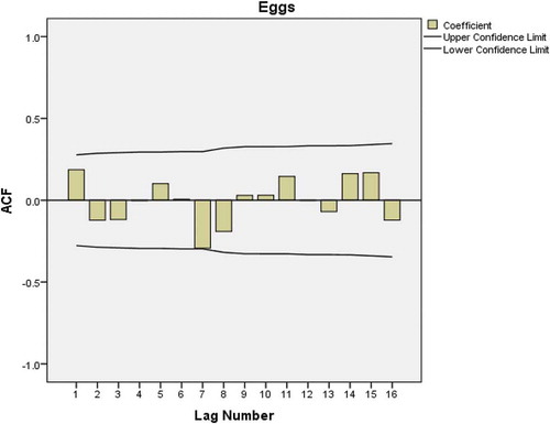
Figure 3. PACF plot after first-order differencing of eggs consumption data.
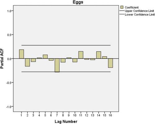
Table 1. Results from SPSS after modeling sample models using eggs consumption data
Figure 4. Residual plots for ACF and PACF after estimating ARIMA(0,1,0) for eggs consumption.
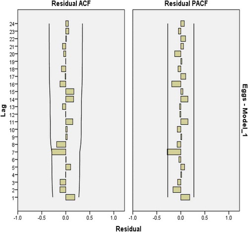
Figure 5. Residual plots for ACF and PACF after estimating ARIMA(1,1,0) for eggs consumption.
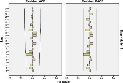
Figure 6. Residual plots for ACF and PACF after estimating ARIMA(0,1,1) for eggs consumption.
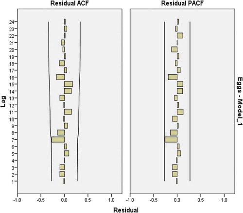
Figure 7. Residual plots for ACF and PACF after estimating ARIMA(1,1,1) for eggs consumption.
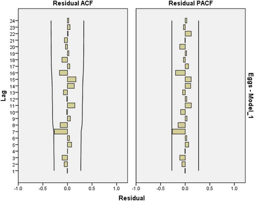
Table 2. Model statistics
Table 3. Model parameter
Table 4. Forecasted data on consumption of eggs
Figure 8. Autocorrelation plot of cattle meat consumption data used to test for stationarity.
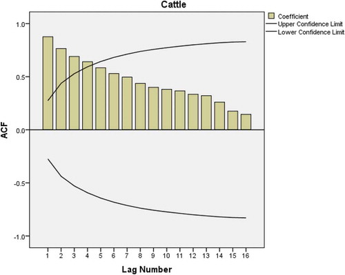
Figure 9. ACF plot after first-order differencing of cattle meat consumption data.
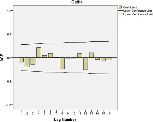
Figure 10. PACF plot after first-order differencing of the cattle meat consumption data.
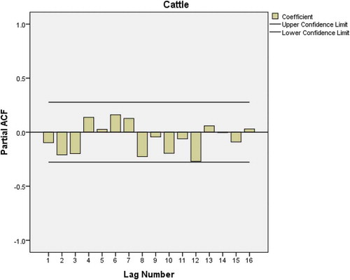
Table 5. Results from SPSS after modeling sample models using cattle meat consumption data
Figure 11. Residual plots for ACF and PACF after estimating ARIMA(0,1,0) for cattle meat consumption.
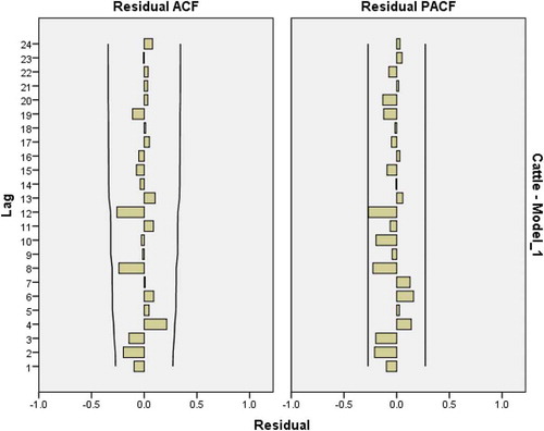
Figure 12. Residual plots for ACF and PACF after estimating ARIMA(1,1,0) for cattle meat for cattle consumption.
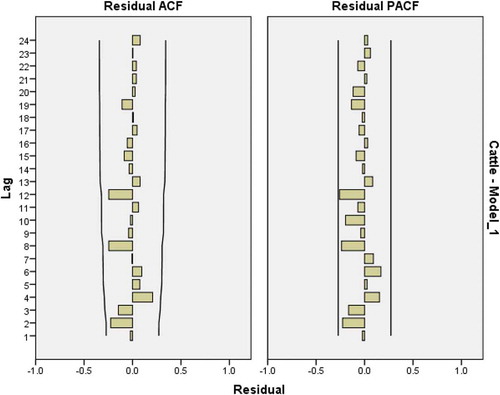
Figure 13. Residual plots for ACF and PACF after estimating ARIMA(0,1,1) for cattle meat consumption.
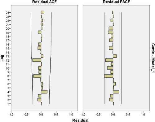
Figure 14. Residual plots for ACF and PACF after estimating ARIMA(1,1,1) for cattle meat consumption.
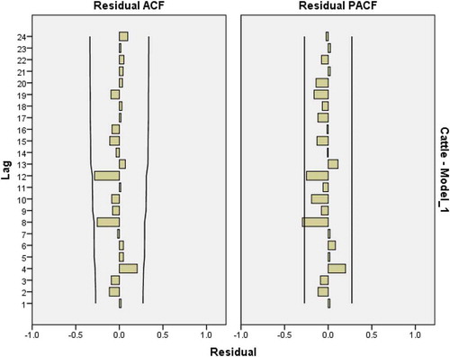
Table 6. Model statistics
Table 7. Model parameters
Table 8. Forecasted data on consumption of cattle meat
Figure 15. Autocorrelation plot of cow milk consumption data used to test for stationarity.
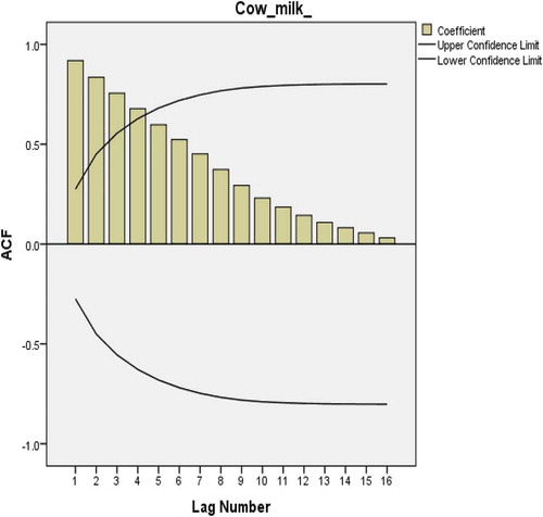
Figure 16. ACF plot after first-order differencing of cow milk consumption data.
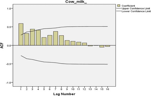
Figure 17. PACF plot after first-order differencing of cow milk consumption data.
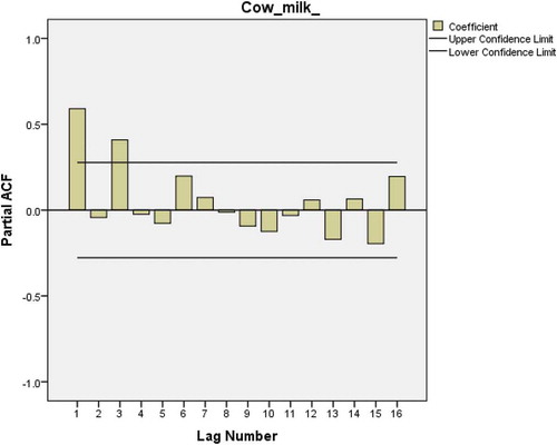
Figure 18. Residual plots for ACF and PACF after estimating ARIMA(1,1,0) for cow milk consumption.
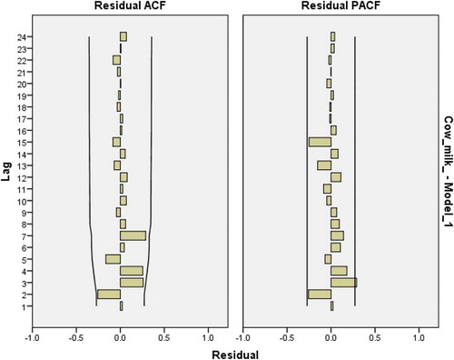
Figure 19. Residual plots for ACF and PACF after estimating ARIMA(3,1,0) for cow milk consumption.
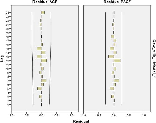
Figure 20. Residual plots for ACF and PACF after estimating ARIMA(3,1,1) for cow milk consumption.
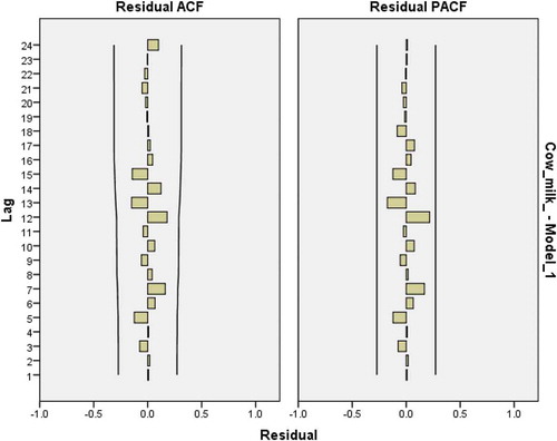
Figure 21. Residual plots for ACFand PACF after estimating ARIMA(2,1,1) for cow milk consumption.
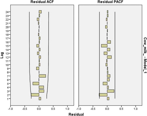
Table 9. Results after modeling sample models from SPSS using cow milk consumption data
Table 10. Model statistics
Table 11. Model parameters results from SPSS for ARIMA(3,1,0) estimated from cow milk consumption data
Table 12. Forecasted data on consumption of cow milk
Figure 22. Autocorrelation plot of chicken meat consumption data used to test for stationarity.
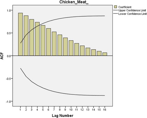
Figure 23. ACF plot after first-order differencing of the chicken meat consumption data.
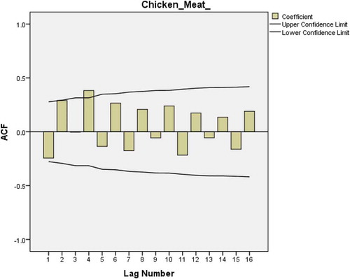
Figure 24. PACF plot after first-order differencing of the chicken meat consumption data.
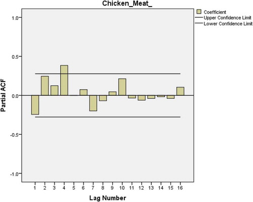
Figure 25. Residual plots for ACF and PACF after estimating ARIMA(0,1,1) for chicken meat consumption.
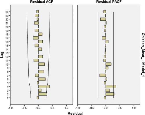
Figure 26. Residual plots for ACF and PACF after estimating ARIMA(0,2,1) for chicken meat consumption.
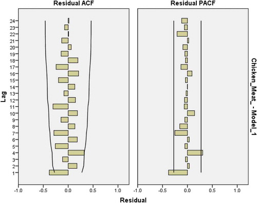
Figure 27. Residual plots for ACF and PACF after estimating ARIMA*(0,2,1) for chicken meat consumption.
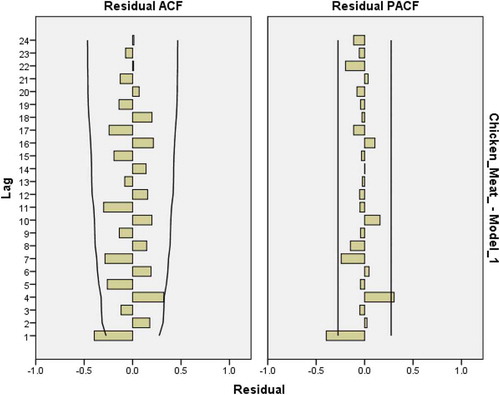
Figure 28. Residual plots for ACF and PACF after estimating BROWN (model) for chicken meatconsumption.
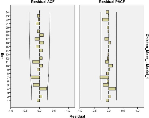
Table 13. Results from SPSS after modeling sample models using chicken meat consumption data
Table 14. SPSS result from BROWN model using chicken meat consumption data
Table 15. Model parameters
Table 16. Forecasted data on consumption of chicken meat
Table 17. ARIMA Model, forecasts and annual rates of growth for livestock products from 2016 to 2020, Tanzania