On the use of intertemporal models to analyse how post-loss and post no-loss insurance demands differ

Figures & data

Figure 1. Insured losses since 1970 (USD billion in 2021 prices). Source: .swiss Re Institute (2021)

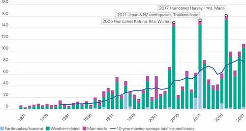
Figure 2. Three dimensional plot of the ratios of premium loading factor to the loss probability.

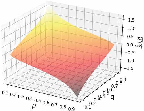
Figure 3. Comparison of loss ($C_2^1$) and no loss ($C_2^2$) against $C_1$.

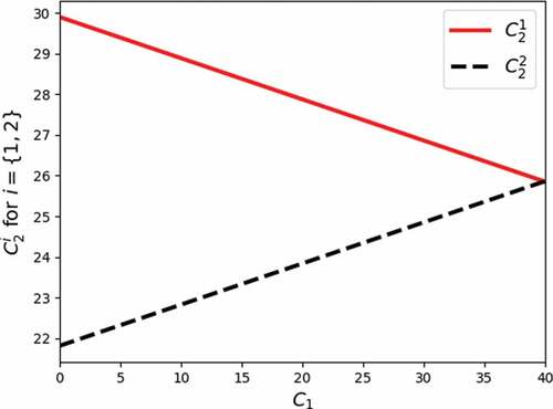
Table 1. Nominal values of the parameter

Parameter	$w_1$	$w$	$L$	$p$	$q$	$R$	$\beta$
Nominal value	$100$	$10$	$40$	$0.4$	$0.5$	$2$	$0.9$

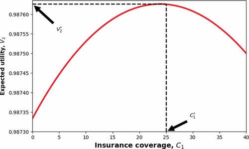
Figure 4. Optimal insurance coverage with intertemporal consideration. The optimal value is at $C_1^{\ast }\approx 24.992$, at which point the greatest expected utility is valued at $V_1^{\ast }\approx 1.8750$. (The interval of $C_1$ over which the plotting is done was subdivided $1,000,000$ times to ensure that an accurate value of the index of $C_1$ is used to obtain the maximum value of $V_1$).

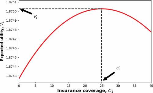
Figure 5. Optimal insurance coverage with intertemporal consideration. The optimal value is at $C_1^{\ast }\approx 24.992$, at which point the greatest expected utility is valued at $V_2^{\ast }\approx 0.98763$.

short-legendGraph 1.

short-legendGraph 2.

Swiss Re Institute (2021). sigma No 1/2021: Natural catastrophes in 2020: secondary perils in the spotlight, but don’t forget primary-peril risks. Retrieved December 20, 2021, from https://www.swissre.com/dam/jcr:ebd39a3b-dc55-4b34-9246-6dd8e5715c8b/sigma-1–2021-en.pdf

 Google Scholar