The Bank of Japan’s equity exchange-traded funds purchasing operation and its impact on equity returns

Figures & data

Figure 1. Central bank assets as a percentage of nominal gross domestic product.

Source: Haver Analytics.

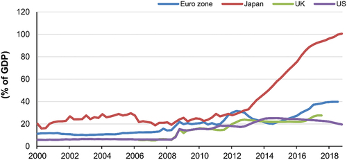
Table 1. Summary statistics for the BoJ’s ETF purchases

	Annual purchasing volume	Purchasing volume over time	Number of purchases per week
	(in trillions of JPY)	(in billions of JPY)
Pre-QQE: 15 December 2010–3 April 2013	No annual target	22.87	0.6
QQE: 4 April 2013–30 October 2014	1	15.74	1.4
QQE2: 31 October 2014–28 July 2016	3	34.85	1.7
Post-QQE2: 29 July 2016–December 31, 2017	6	71.43	1.5

Source: The Bank of Japan.

Figure 2. The BoJ’s exchange-traded fund (ETF) purchasing volume over time, 2010–2018.

Note. The BoJ started ETF purchases on 15 December 2010. Before the BoJ introduced the quantitative and qualitative easing (QQE) on 4 April 2013, no annual purchasing targets existed. The annual purchasing target was ¥1 trillion between 4 April 2013 and 30 October 2014; ¥3 trillion between 31 October 2014 and 28 July 2016; and ¥6 trillion after 29 July 2016.

Source: The Bank of Japan.

Figure 3. Composition of the BoJ’s ETF purchases, 2012–2017.

Note. The BoJ’s ETF purchases were initially linked to both the Nikkei225 and the Topix and were subsequently expanded on 31 October 2014, to influence the JPX400 ETFs. The amount of each ETF purchase was proportional to the total market capitalization of each ETF. This figure indicates my estimation of the composition of the BoJ’s ETF purchases based on market capitalization data.

Sources: Bloomberg Finance LP, the Bank of Japan.

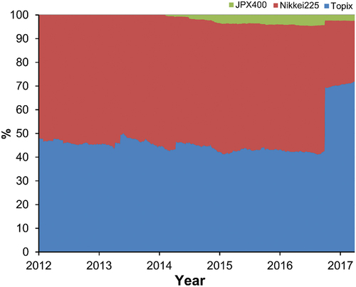
Table 2. Descriptive statistics based on the BoJ’s ETF purchases

		N	mean	sd	Min	max
Day without BoJ purchases
fx_day	USD/JPY daily return	1,369	0.136	0.557	−2.377	4.601
sp	S&P500 daily return	1,333	0.086	0.844	−4.782	4.332
tpx	Topix daily return	1,277	0.434	1.041	−3.256	8.021
nky	Nikkei225 daily return	1,386	0.42	1.081	−3.959	7.709
fx_am	USD/JPY half-day return (AM)	1,367	0.14	0.514	−2.135	4.417
tpx_am	Topix half-day return (AM)	1,276	0.441	0.795	−1.528	5.967
nky_am	Nikkei225 half-day return (AM)	1,277	0.46	0.856	−1.595	5.706
fx_pm	USD/JPY half-day return (PM)	1,374	−0.004	0.196	−2.695	1.762
tpx_pm	Topix half-day return (PM)	1,277	−0.007	0.572	−4.651	3.056
nky_pm	Nikkei225 half-day return (PM)	1,277	−0.005	0.605	−5.005	3.334
Day with BoJ purchases
fx_day	USD/JPY daily return	451	−0.334	0.573	−2.742	2.335
sp	S&P500 daily return	439	−0.069	1.016	−6.663	4.741
tpx	Topix daily return	452	−1.04	1.272	−9.473	2.711
nky	Nikkei225 daily return	452	−1.078	1.343	−10.554	2.203
fx_am	USD/JPY half-day return (AM)	451	−0.323	0.516	−2.645	1.715
tpx_am	Topix half-day return (AM)	452	−1.057	0.897	−6.973	0.037
nky_am	Nikkei225 half-day return (AM)	452	−1.051	0.921	−6.452	0.45
fx_pm	USD/JPY half-day return (PM)	452	−0.012	0.25	−1.483	2.635
tpx_pm	Topix half-day return (PM)	452	0.015	0.738	−5.853	3.969
nky_pm	Nikkei225 half-day return (PM)	452	−0.029	0.833	−7.527	3.995
Total
Day with BoJ purchases
fx_day	USD/JPY daily return	1,820	0.02	0.597	−2.742	4.601
sp	S&P500 daily return	1,772	0.047	0.892	−6.663	4.741
tpx	Topix daily return	1,729	0.049	1.281	−9.473	8.021
nky	Nikkei225 daily return	1,838	0.052	1.319	−10.554	7.709
fx_am	USD/JPY half-day return (AM)	1,818	0.025	0.552	−2.645	4.417
tpx_am	Topix half-day return (AM)	1,728	0.05	1.053	−6.973	5.967
nky_am	Nikkei225 half-day return (AM)	1,729	0.065	1.097	−6.452	5.706
fx_pm	USD/JPY half-day return (PM)	1,826	−0.006	0.211	−2.695	2.635
tpx_pm	Topix half-day return (PM)	1,729	−0.002	0.62	−5.853	3.969
nky_pm	Nikkei225 half-day return (PM)	1,729	−0.011	0.672	−7.527	3.995

Source: Bloomberg Finance LP.

Figure 4. Historical charts for the Nikkei225, Topix, S&P500, and USD/JPY, 2010–2019.

Sources: Bloomberg Finance LP and the Bank of Japan.

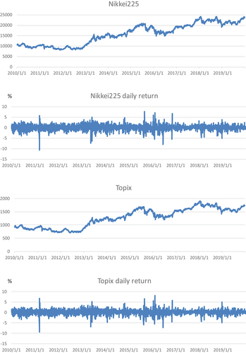
Figure 4. Continued.

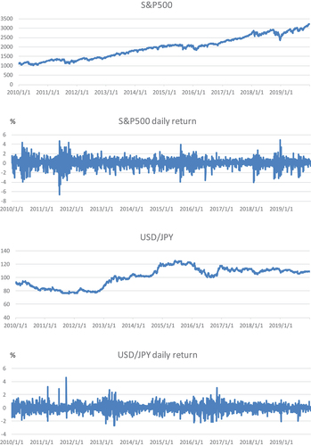
Table 3. Estimation results of simple OLS regression Equation (1)(1) $\mathrm{\Delta }{\mathit{s}}_{\mathit{t}}\hspace{0.17em}=\hspace{0.17em}{\mathit{\alpha }}_0+\hspace{0.17em}{\mathit{\alpha }}_{\mathbf{1}}\mathbf{\ast }\mathrm{\Delta }\mathit{s}{\mathit{p}}_{\mathit{t}\mathbf{-}\mathbf{1}}\hspace{0.17em}+{\mathit{\alpha }}_{\mathbf{2}}\mathbf{\ast }\mathrm{\Delta }\mathit{f}{\mathit{x}}_{\mathit{t}}\hspace{0.17em}+\hspace{0.17em}{\mathit{\alpha }}_{\mathbf{3}}\mathbf{\ast }\mathit{b}\mathit{o}{\mathit{j}}_{\mathit{t}}\hspace{0.17em}+{\mathit{\epsilon }}_{\mathit{t}}$(1)

	nky			tpx
	Full sample	Before QQE	After QQE	Full sample	Before QQE	After QQE
sp [−1]	0.464***	0.360***	0.480***	0.459***	0.339***	0.510***
	(0.0377)	(0.0475)	(0.0595)	(0.0371)	(0.0448)	(0.0570)
Fx	0.982***	0.580***	1.141***	0.958***	0.751***	1.137***
	(0.0760)	(0.127)	(0.0801)	(0.0784)	(0.115)	(0.0740)
boj	−0.00916***	−0.0484***	−0.00687***	−0.00823***	−0.0489***	−0.00555***
	(0.00122)	(0.00703)	(0.00123)	(0.00125)	(0.00610)	(0.00124)
Constant	0.0948***	0.134**	0.102**	0.0783**	0.166***	0.0750*
	(0.0261)	(0.0421)	(0.0328)	(0.0266)	(0.0396)	(0.0322)
N	1756	563	1193	1657	770	1125
R-sq	0.428	0.395	0.478	0.433	0.427	0.506
adj. R-sq	0.427	0.391	0.476	0.432	0.425	0.504
Sample period	12/15/2010–12/29/2017	12/15/2010–4/3/2013	4/4/2013–12/29/2017	12/15/2010–12/29/2017	12/15/2010–4/3/2013	4/4/2013–12/29/2017

Standard errors appear in parentheses. * p < 0.05, ** p < 0.01, *** p < 0.001.

Note. This table reports the results of OLS regressions of daily equity index returns. The dependent variable is the Nikkei 225 daily return (nky) or Topix daily return (tpx). “sp[−1]” denotes the previous day’s S&P 500 returns, “fx” is the USD/JPY returns from 3:00 p.m. the previous day to 3:00 p.m. the current day, and “boj” is the BoJ’s ETF purchasing volume (in billions of yen).

Table 4. Estimation probit model results Equation (2)(2) $Pr\left(BoJ\hspace{0.17em}purchasesETF\right)=\mathrm{\Phi }\left({\alpha }_0+{\alpha }_1\ast \mathrm{\Delta }{s}_{am,\hspace{0.17em}t}\right)+{\text{isin}}_t$(2)

	1 if BoJ purchases ETF, zero if not
	Full sample	Before QQE	After QQE	Full sample	Before QQE	After QQE
nky_am	−1.752***	−2.943***	−2.340***
	(0.0887)	(0.339)	(0.143)
tpx_am				−2.263***	−4.675***	−3.499***
				(0.117)	(0.621)	(0.219)
Constant	−1.092***	−3.395***	−0.826***	−1.244***	−4.810***	−1.046***
	(0.0544)	(0.365)	(0.0640)	(0.0633)	(0.601)	(0.0806)
N	1729	565	1164	1729	565	1164
pseudo R-sq	0.473	0.708	0.542	0.541	0.806	0.651
Sample period	12/15/2010–12/29/2017	12/15/2010–4/3/2013	4/4/2013–12/29/2017	12/15/2010–12/29/2017	12/15/2010–4/3/2013	4/4/2013–12/29/2017

Standard errors appear in parentheses. * p < 0.05, ** p < 0.01, *** p < 0.001.

Note. This table reports the results of the probit model for estimating the BoJ’s ETF purchases. The dependent variable is a binary variable that takes the value of one if the BoJ purchases ETFs and zero otherwise. “nky_am”, and “tpx_am” denote the Nikkei 225 and Topix returns in the morning session, respectively.

Figure 5. Estimated probability of the BoJ’s ETF purchases using the probit model.

Estimated by using the following probit model:$Pr\left(BoJ\hspace{0.17em}purchases\hspace{0.17em}ETF\right)=\left({\alpha }_0+{\alpha }_1\ast \mathrm{\Delta }{s}_{am,\hspace{0.17em}t}\right)+{\text{isin}}_t$where ∆s_am,t are returns in the morning session of the Topix, and Ф is a cumulative standard normal distribution. “Before QQE” is from 15 December 2010 to 3 April 2013, and “After QQE” is from April 4 to 29 December 2017.

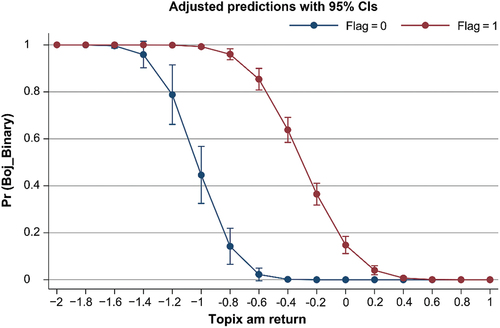
Table 5. Predictive power of the probit model

Sample period: 15 December 2010–3 April 2013 (before QQE)				Sample period: 4 April 2013–29 December 2017 (after QQE)
	TRUE				TRUE
Classified	D	~D	Total	Classified	D	~D	Total
+	68	0	68	+	309	33	342
−	2	495	497	−	73	748	821
Total	70	495	565	Total	382	781	1163
Classified + if predicted Pr(D)≥ 0.5				Classified + if predicted Pr(D)≥ .5
True D defined as if BoJ purchases ETF				True D defined as if BoJ purchases ETF
Sensitivity	Pr(+|D)	97.14%		Sensitivity	Pr(+|D)	80.89%
Specificity	Pr(−|~D)	100.00%		Specificity	Pr(−|~D)	95.77%
Positive predictive value	Pr(D|+)	100.00%		Positive predictive value	Pr(D|+)	90.35%
Negative predictive value	Pr(~D|−)	99.60%		Negative predictive value	Pr(~D|−)	91.11%
False + rate for true ~D	Pr(+|~D)	0.00%		False + rate for true ~D	Pr(+|~D)	4.23%
False − rate for true D	Pr(−|D)	2.86%		False − rate for true D	Pr(−|D)	19.11%
False + rate for classified +	Pr(~D|+)	0.00%		False + rate for classified +	Pr(~D|+)	9.65%
False − rate for classified −	Pr(D|−)	0.40%		False − rate for classified −	Pr(D|−)	8.89%
Correctly classified		99.65%		Correctly classified		90.89%

Note. TRUE D: The BoJ purchases ETFs, True ~D: The BoJ does not purchase ETFs, Classified +: The model predicts the BoJ’s ETF purchases, Classified -: The model does not predict the BoJ’s ETF purchases.

Figure 6. Assumed timeframe for the BoJ’s ETF purchasing operation.

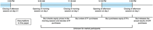
Table 6. OLS regression results for afternoon returns Equation (3)

	nky_pm			tpx_pm
	Full sample	Before QQE	After QQE	Full sample	Before QQE	After QQE
nky_am	0.0967***	0.164***	0.0839***
	(0.0254)	(0.0586)	(0.0253)
tpx_am				0.0882***	0.130***	0.0885***
				(0.0240)	(0.0494)	(0.0264)
fx_pm	1.775***	1.048***	1.927***	1.587***	1.028***	1.707***
	(0.147)	(0.190)	(0.173)	(0.124)	(0.168)	(0.144)
boj	0.00317***	0.0106***	0.00311***	0.00377***	0.0116***	0.00386***
	(0.000668)	(0.00381)	(0.000624)	(0.000610)	(0.00348)	(0.000612)
Constant	−0.0378**	−0.0262	−0.0585***	−0.0337**	−0.0220	−0.0558***
	(0.0164)	(0.0283)	(0.0200)	(0.0151)	(0.0253)	(0.0191)
N	1723	559	1164	1722	559	1163
R-sq	0.349	0.16	0.423	0.331	0.137	0.406
adj. R-sq	0.348	0.156	0.421	0.330	0.132	0.404
Sample period	12/15/2010–12/29/2017	12/15/2010–4/3/2013	4/4/2013–12/29/2017	12/15/2010–12/29/2017	12/15/2010–4/3/2013	4/4/2013–12/29/2017

Standard errors appear in parentheses. * p < 0.05, ** p < 0.01, *** p < 0.001.

Note. This table reports the results of OLS regressions of equity index returns for the afternoon session. The dependent variable is afternoon session returns for the Nikkei 225 (nky_pm) or Topix (tpx_pm). “nky_am” and “tpx_am” are morning session returns for Nikkei 225 and Topix. “fx_pm” is USD/JPY returns from 11:30 a.m. to 3:00 p.m. “boj” is the BoJ’s ETF purchasing volume (in billions of yen).

Table 7. Impact of expected and unexpected ETF purchases by the BoJ Equation (4)(4) $\mathrm{\Delta }{\mathit{s}}_{\mathit{p}\mathit{m},\mathit{t}}\hspace{0.17em}=\hspace{0.17em}{\mathit{\alpha }}_0+\hspace{0.17em}{\mathit{\alpha }}_{\mathbf{1}}\mathbf{\ast }\mathrm{\Delta }{\mathit{s}}_{\mathit{a}\mathit{m},\mathit{t}}\hspace{0.17em}+{\mathit{\alpha }}_{\mathbf{2}}\mathbf{\ast }\mathrm{\Delta }\mathit{f}{\mathit{x}}_{\mathit{p}\mathit{m},\mathit{t}}\hspace{0.17em}+\hspace{0.17em}{\mathit{\alpha }}_{\mathbf{3}}\mathbf{\ast }\mathit{b}\mathit{o}{\mathit{j}}_{\mathit{e}\mathit{x}\mathit{p},\mathit{t}}+{\mathit{\alpha }}_{\mathbf{4}}\mathbf{\ast }\mathit{b}\mathit{o}{\mathit{j}}_{\mathit{u}\mathit{n}\mathit{e}\mathit{x}\mathit{p},\mathit{t}}\hspace{0.17em}+{\mathit{\epsilon }}_{\mathit{t}}$(4)

	nky_pm	tpx_pm
nky_am	0.0761***
	(0.0257)
tpx_am		0.0784***
		(0.0271)
fx_pm	1.926***	1.705***
	(0.172)	(0.144)
boj_exp	0.00181	0.00232*
	(0.00144)	(0.00121)
boj_unexp	0.00341***	0.00420***
	(0.000616)	(0.000626)
Constant	0.0538***	0.0502***
	(0.0197)	(0.0189)
N	1164	1163
# of expected purchases	176	176
# of unexpected purchases	206	206
R-sq	0.423	0.407
adj. R-sq	0.421	0.405
Sample period	4/4/2013- 12/29/2017	4/4/2013- 12/29/2017

Standard errors appear in parentheses. * p < 0.05, ** p < 0.01, *** p < 0.001.

Note. This table reports the results of OLS regressions of equity index returns for the afternoon session. The dependent variable is Nikkei 225 returns (nky_pm) or Topix returns (tpx_pm). “nky_am” and “tpx_am” are morning session returns for the Nikkei 225 and the Topix. “fx_pm” is USD/JPY returns from 11:30 a.m. to 3:00 p.m. “boj_exp” and “boj_unexpt” represent expected and unexpected ETF purchasing volume, respectively, by the BoJ (in billions of yen).

Table 8. OLS regression results for returns reversals Equation (5)(5) $\mathbf{\Delta }{s}_{am,t}={\alpha }_0+{\alpha }_1\ast \mathrm{\Delta }{s}_{pm,t-1}+{\alpha }_2\ast \mathrm{\Delta }f{x}_{am,t}+{\alpha }_3\ast \mathrm{\Delta }s{p}_{t-1}+{\alpha }_4\ast bo{j}_{unexp,t-1}+{\epsilon }_t$(5)

	nky_am	tpx_am
nky_pm[−1]	−0.266***
	(0.0463)
tpx_pm[−1]		−0.222***
		(0.0535)
fx_am	1.085***	1.023***
	(0.0524)	(0.0509)
sp[−1]	0.558***	0.545***
	(0.0458)	(0.0434)
boj_unexp[−1]	−0.00228**	−0.00244***
	(0.000897)	(0.000875)
Constant	0.0415*	0.0305
	(0.0235)	(0.0224)
N	1070	1069
R-sq	0.599	0.594
adj. R-sq	0.597	0.592
Sample period	4/4/2013–12/29/2017	4/4/2013–12/29/2017

Standard errors appear in parentheses. * p < 0.05, ** p < 0.01, *** p < 0.001.

Note. This table reports the results of OLS regressions of equity index returns for the morning session. The dependent variable is the morning session returns for the Nikkei 225 (nky_am) or the Topix (tpx_am). “nky_pm[−1]” and “tpx_pm[−1]” are afternoon session returns for the Nikkei 225 and the Topix the previous day. “fx_am” is USD/JPY returns from 3:00 p.m. the previous day to 11:30 a.m. the current day. “sp[−1]” is S&P500 returns the previous day. “boj_unexpt[−1]” is the unexpected ETF purchasing volume (in billions of yen) the previous day.

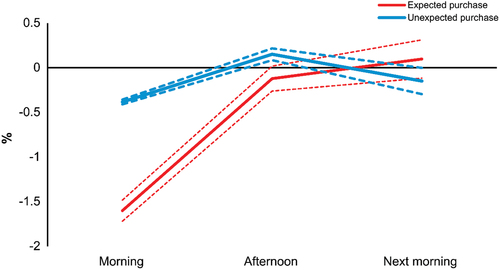
Figure 7. Topix returns when the BoJ purchases ETFs.

Note. The dotted lines represent 95% confidence intervals. This paper defines ETF purchases with a probability higher than 95% in the probit model, as expected, and those with a probability lower than 95%, as unexpected. When the BoJ conducts expected ETF purchases, Topix returns are negative in the afternoon session and approximately zero in the next day’s morning session. In contrast, when the BoJ conducts unexpected purchases, Topix returns are positive in the afternoon session and negative in the next day’s morning session.