Greenspan’s adherence to the Taylor rule: examining Federal Reserve chairmen policy regimes and deviations from the Taylor rule

Figures & data

Figure 1. St. Louis fed Taylor rule.

Notes: The figure shows the federal funds rate (red), along with the implied federal funds rate from the original formulation of the Taylor Rule (blue), as calculated by The St. Louis Federal Reserve. The vertical bars denote recessions as defined by the NBER. Both series are based on quarterly data, with the federal funds rate data points representing the quarterly average of the effective federal funds rate.

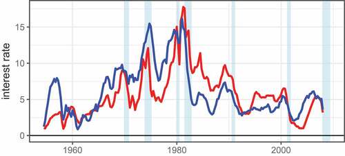
Figure 2. $i_{FedFund,t}-i_{Taylor,t}:$1954–2008.

Notes: The figure shows the difference between the quarterly average federal funds rate, $i_{FedFund}$ and the federal funds rate implied by the Taylor Rule, $i_{Taylor}$. The series is quarterly from 1954:Q3 to 2008:Q1.

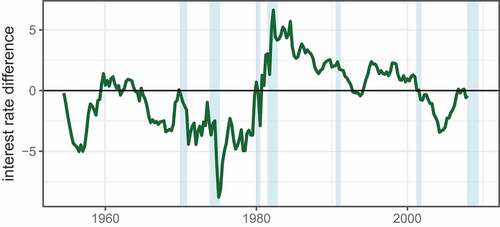
Table 1. Summary of literature review on identifying and analyzing monetary policy regimes

Methodology	Features	References
Binary variable method	Limited to only two regimes and did not account for changes in the economy over time	Hamilton (1989)
Structural VAR	Allow for multiple regimes, but still assumed a fixed and known number of regimes	Sims (1992), Judd and Rudebusch (1998), Clarida et al. (1999), Fair (2001), Sims and Zha (2006)
Time-varying parameter models	Allow for changes in the model parameters over time, but have their own limitations	Primiceri (2005), Boivin (2006)
Bayesian methods	Allow for more flexible modeling of uncertainty and can produce more accurate estimates of the model parameters but require specifying prior distributions for the model parameters	Timothy and Sargent (2005), Murray et al. (2015) and Alba and Wang (2017)
Structural change model with regime switching	Identify regimes and fit OLS regressions for each regime.	Alex et al. (2019)
Machine learning methods	Use methods such as sentiment analysis, neural network and topic modelling to estimate changes in monetary policy regimes, allowing for more flexible modeling of complex relationships between variables.	Shapiro and Wilson (2022), Handlan (2021), and Hansen and McMahon (2016)

Figure 3. Gap version of Okun’s law 1954–2008.

Notes: The figure shows the regression results based on Equation 4(4) $y_t=-c(U_t-U_t^{\ast }).$(4) , regressing the Output gap on the Unemployment gap using quarterly Output and Unemployment. The estimated slope for the period is −1.26, rather that the −2 estimated from Okun’s original data.

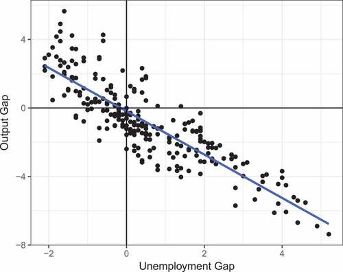
Figure 4. Monthly natural rate of unemployment.

Notes: The figure displays the U.S. Congressional Budget Office Short-Term Natural Rate of Unemployment, $U_t^{\ast }$, interpolated from quarterly to monthly frequency.

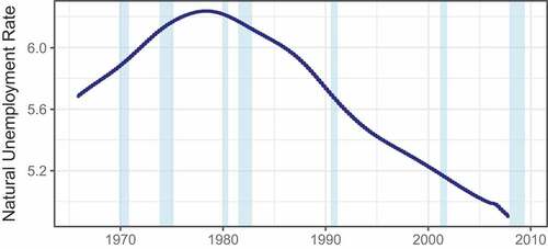
Figure 5. Real-Time $i_{FedFund,t}-i_{St.Louis,t}$, 1965–2008.

Notes: The figure shows the difference between the monthly average federal funds rate, $i_{FedFund}$ and the federal funds rate implied by the monthly version of the Taylor Rule, $i_{TaylorMonthly}$, in Equation 6(6) $i_t=2+{\pi }_t-0.63(U_t-U_t^{\ast })+0.5({\pi }_t-2).$(6) . The inflation and unemployment estimates are the initial series available at the time of the Federal Reserve meeting, acquired from the Federal Reserve Bank of Philadelphia’s Real-Time Data Set, rather than the revised series published by St. Louis Federal Reserve. The series runs from October 1965 to December 2007.

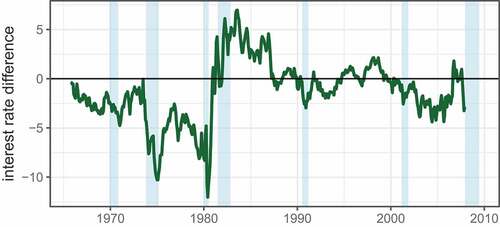
Table 2. Tukey HSD:St. Louis rule

	Difference	Lower	Upper	P-value
Bernanke-Greenspan	−0.835	−1.703	0.034	0.069
Burns-Greenspan	−2.990	−3.861	−2.118	0
Martin-Greenspan	−1.218	−2.309	−0.127	0.017
Miller-Greenspan	−4.450	−6.198	−2.701	0
Volcker-Greenspan	2.568	1.696	3.439	0
Burns-Bernanke	−2.155	−3.182	−1.128	0.00000
Martin-Bernanke	−0.383	−1.602	0.835	0.968
Miller-Bernanke	−3.615	−5.446	−1.785	0.00000
Volcker-Bernanke	3.402	2.375	4.429	0
Martin-Burns	1.772	0.551	2.992	0.0004
Miller-Burns	−1.460	−3.292	0.372	0.219
Volcker-Burns	5.557	4.528	6.587	0
Miller-Martin	−3.232	−5.178	−1.286	0.00002
Volcker-Martin	3.785	2.565	5.006	0
Volcker-Miller	7.017	5.185	8.849	0

Notes: The table shows the results of the Tukey Honest Significant Difference multiple comparison procedure for testing the difference in mean Federal Reserve Chairman deviance from the original version of the Taylor Rule. Greenspan has a significantly tighter adherence to the Taylor Rule than every former Chairman other than Bernanke.

Table 3. Tukey HSD: Bernanke rule

	Difference	Lower	Upper	P-value
Bernanke-Greenspan	0.297	−0.636	1.231	0.965
Burns-Greenspan	−2.475	−3.412	−1.538	0
Martin-Greenspan	−2.341	−3.513	−1.168	0.00000
Miller-Greenspan	−4.222	−6.101	−2.342	0
Volcker-Greenspan	3.974	3.037	4.911	0
Burns-Bernanke	−2.773	−3.876	−1.669	0
Martin-Bernanke	−2.638	−3.948	−1.328	0.00000
Miller-Bernanke	−4.519	−6.487	−2.551	0
Volcker-Bernanke	3.676	2.573	4.780	0
Martin-Burns	0.135	−1.178	1.447	1.000
Miller-Burns	−1.747	−3.716	0.223	0.121
Volcker-Burns	6.449	5.342	7.556	0
Miller-Martin	−1.881	−3.973	0.211	0.110
Volcker-Martin	6.314	5.002	7.627	0
Volcker-Miller	8.196	6.226	10.165	0

Notes: The table shows the results of the Tukey Honest Significant Difference multiple comparison procedure for testing the difference in mean Federal Reserve Chairman deviance from the Bernanke version of the Taylor Rule. Again, Greenspan has a significantly tighter adherence to the rule than every former Chairman besides Bernanke.

Figure 6. Fitted regimes with Fed Chairman tenure periods, 1965–2008.

Notes: The figure shows the monthly series representing the monthly deviation from the Taylor Rule (green), along with the conditional means from the Bai and Perron structural break methodology (brown). The tenure of each Federal Reserve chairman is represented by the shaded background regions. Martin (pink), Burns (salmon), Volcker (yellow), Greenspan (tan), Bernanke (light blue), and Yellen (dark blue) are denoted. Vertical grey bars represent the NBER recession periods.

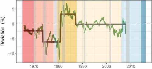
Figure 7. Fitted Regimes using PCE rather than CPI inflation target from 2000 to 2008.

Notes: The figure shows the monthly series representing the monthly deviation from the Taylor Rule (green) corrected for the use of PCE as the preferred measure of inflation beginning in 2000, along with the conditional means from the Bai and Perron structural break methodology (brown). The tenure of each Federal Reserve chairman is represented by the shaded background regions. Martin (pink), Burns (salmon), Volcker (yellow), Greenspan (tan), Bernanke (light blue), and Yellen (dark blue) are denoted. Vertical grey bars represent the NBER recession periods.

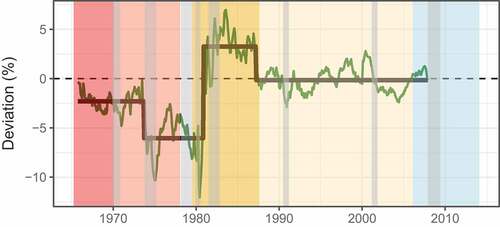
Figure 8. Fitted regimes using university of michigan 1-year inflation expectations for the inflation gap rather than CPI or PCE from 1982 to 2015.

Notes: The figure shows the monthly series representing the monthly deviation from the Taylor Rule (green) using the University of Michigan 1-year inflation expectations survey to calculate the inflation gap, along with the two conditional means from the Bai and Perron structural break methodology (brown). The tenure of each Federal Reserve chairman is represented by the shaded background regions. Martin (pink), Burns (salmon), Volcker (yellow), Greenspan (tan), Bernanke (light blue), and Yellen (dark blue) are denoted. Vertical grey bars represent the NBER recession periods.

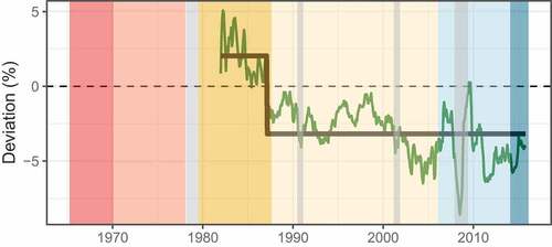
Figure 9. Markov Switching: Regime 0 (“Loose”).

Notes: The figure shows the periods corresponding to the third Markov switching regime conditional mean and variance for the deviations from the Taylor Rule. The fitted conditional mean and variance are −1.856 and 0.764, respectively. This regime can be interpreted as “loose” regime, where the federal funds rate is lower than the recommendation from the Taylor Rule. Periods of the Martin, Burns, and Greenspan chairmanships correspond to this regime.

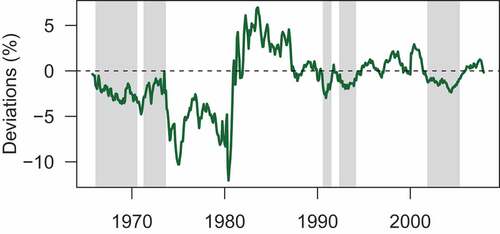
Figure 10. Markov switching: regime 1 (“Tight”).

Notes: The figure shows the periods corresponding to the first Markov switching regime conditional mean and variance for the deviations from the Taylor Rule. The fitted conditional mean and standard deviation are 0.358 and 0.722, respectively. This regime can be interpreted as “tight” regime, where the federal funds rate is higher than the recommendation from the Taylor Rule. Periods of the Greenspan and Bernanke chairmanships correspond to this regime.

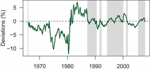
Figure 11. Markov switching: regime 2 (“Inconsistent”).

Notes: The figure shows the periods corresponding to the second Markov switching regime conditional mean and variance for the deviations from the Taylor Rule. The fitted conditional mean and standard deviation are −1.546 and 4.930, respectively. This regime can be interpreted as a non-standard regime, periods where monetary policy substantially deviates from the Taylor rule. The period covers the Burns chairmanship keeping monetary policy loose at Nixon’s behest, and the Volcker chairmanship keeping monetary policy tighter than recommended due to the emphasis on fighting inflation over boosting output during his tenure. Most of Burns and all of Volcker’s tenure deviate substantially from the real-time Taylor Rule. A small portion of the Greenspan’s chairmanship post-2000 is “inconsistent” with the Taylor Rule, but he appears to have erred in being overly tight, based on the plot, rather than too loose.

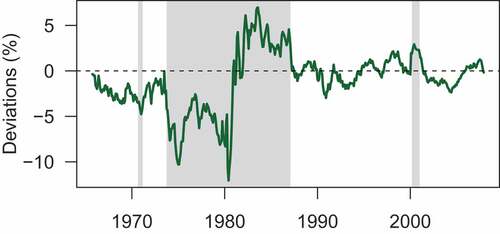
Figure 12. Clustering results of FOMC transcripts: 2 clusters.

Notes: The figure shows the clustering results when the FOMC transcripts are divided into 2 clusters. We interpret each cluster of similar texts as a distinct regime of monetary policy.

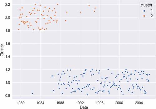
Table 4. Mean deviation from the Taylor rule: By clusters

Cluster	Mean deviation	Mean deviation	Mean deviation
	two clusters	three clusters	four clusters
Cluster 1	−0.021	−0.021	−0.021
Cluster 2	2.93	3.72	3.44
Cluster 3	-	0.557	2.54
Cluster 4	-	-	0.557

Notes: The table shows the mean deviation from the Taylor for each cluster in the case of two, three, and four clusters.

Figure 13. Clustering results of FOMC transcripts: 3 clusters.

Notes: The figure shows the clustering results when the FOMC transcripts are divided into 3 clusters. We interpret each cluster of similar texts as a distinct regime of monetary policy.

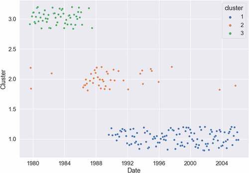
Figure 14. Clustering results of FOMC transcripts: 4 clusters.

Notes: The figure shows the clustering results when the FOMC transcripts are divided into 4 clusters. We interpret each cluster of similar texts as a distinct regime of monetary policy.

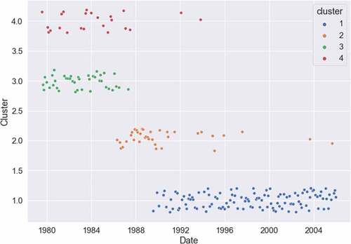
Figure 15. Clustering results of FOMC transcripts: 5 clusters.

Notes: The figure shows the clustering results when the FOMC transcripts are divided into 5 clusters. We interpret each cluster of similar texts as a distinct regime of monetary policy.

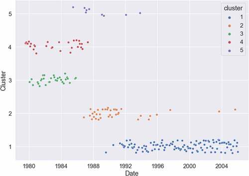
Figure 16. Wordcloud of the top texts in cluster 1 (regime from roughly from 1990 to 2007).

Notes: The figure shows the wordcloud for the top single word and two-word phrases in the first cluster. The transcripts from the later era of Greenspan’s tenure paid close attention to U.S. stock market and financial sector in general.

Figure 17. Wordcloud of the top texts in cluster 2 (regime from roughly from 1987 to 1990).

Notes: The figure shows the wordcloud for the top single word and two-word phrases in the second cluster. This cluster corresponds mostly to texts early in Greenspan’s tenure, where international trade and exchange rates relative to U.S. dollar figured prominently in the conversation.

Figure 18. Wordcloud of the top texts in cluster 3 (regime from roughly from 1979 to 1986).

Notes: The figure shows the wordcloud for the top single word and two-word phrases in the third cluster. This cluster corresponds mostly to texts in Volcker’s tenure, where the transcripts reflect the debate over the use of money supply or federal funds rate as targets, as well as the desire to reduce unemployment.

Figure A1. Within Groups Sums of Squares.

Hamilton, J. D. (1989). A new approach to the economic analysis of nonstationary time series and the business cycle. Econometrica: Journal of the Econometric Society, 57(2), 357–384. https://doi.org/10.2307/1912559

 Web of Science ®Google Scholar

Sims, C. A. (1992). Interpreting the macroeconomic time series facts: The effects of monetary policy. European Economic Review, 36(5), 975–1000.

 Web of Science ®Google Scholar

Judd, J. P., & Rudebusch, G. D. (1998). Taylor’s rule and the fed: 1970-1997. Economic Review–Federal Reserve Bank of San Francisco, 3, 3–16.

 Google Scholar

Clarida, R., Gali, J., & Gertler, M. (1999). The science of monetary policy: A new Keynesian perspective. Journal of Economic Literature, 37(4), 1661–1707. https://doi.org/10.1257/jel.37.4.1661

 Web of Science ®Google Scholar

Fair, R. C. (2001). Actual federal reserve policy behavior and interest rate rules. Federal Reserve Bank of New York Economic Policy Review, 7(1), 61–72.

 Google Scholar

Sims, C. A., & Zha, T. (2006). Were there regime switches in US monetary policy? The American Economic Review, 96(1), 54–81.

 Web of Science ®Google Scholar

Primiceri, G. E. (2005). Time varying structural vector autoregressions and monetary policy. The Review of Economic Studies, 72(3), 821–852.

 Web of Science ®Google Scholar

Boivin, J. (2006). Has US monetary policy changed? Evidence from drifting coefficients and real-time data. Journal of Money, Credit, and Banking, 38(7), 1149–1173. https://doi.org/10.1353/mcb.2006.0065

 Google Scholar

Timothy, C., & Sargent, T. J. (2005). Drifts and volatilities: Monetary policies and outcomes in the post WWII US. Review of Economic Dynamics, 8(2), 262–302. https://doi.org/10.1016/j.red.2004.10.009

 Web of Science ®Google Scholar

Murray, C. J., Nikolsko-Rzhevskyy, A., & Papell, D. H. (2015). Markov switching and the Taylor principle. Macroeconomic Dynamics, 19(4), 913–930.

 Web of Science ®Google Scholar

Alba, J. D., & Wang, P. (2017). Taylor rule and discretionary regimes in the United States: Evidence from a k-state Markov regime-switching model. Macroeconomic Dynamics, 21(3), 817–24. https://doi.org/10.1017/S1365100515000693

 Web of Science ®Google Scholar

Alex, N.R., Papell, D. H., & Prodan, R. (2019). The Taylor principles. Journal of Macroeconomics, 62, 103159.

 Web of Science ®Google Scholar

Shapiro, A. H., & Wilson, D. J. (2022). Taking the fed at its word: A new approach to estimating central bank objectives using text analysis. The Review of Economic Studies, 89(5), 2768–2805.

 Web of Science ®Google Scholar

Handlan, A. (2021). Text shocks and monetary surprises (Doctoral dissertation, University of Minnesota).

 Google Scholar

Hansen, S., & McMahon, M. (2016). Shocking language: Understanding the macroeconomic effects of central bank communication. Journal of International Economics, 99, S114–133. https://doi.org/10.1016/j.jinteco.2015.12.008

 Web of Science ®Google Scholar