How justified is abandoning money from monetary policy? Evidence from dynamically simulated ARDL

Figures & data

Table 1. The table depicts a review of the empirical literature on MDF and its stability and covers the authors’ details, countries, sample covered, methodology, and findings of the studies

Studies	Countries, sample covered	Methodology	Conclusion
Moosa (1992)	India, 1972Q1-1990Q4	Unit root tests, EG, AEG, CRDW, and JJ cointegration tests	Stable M1 and unstable M2
Arrau and De Gregorio (1993)	Chile, 1975Q1-1989Q4 and Mexico, 1980Q1-1989Q3	Unit root test and cointegration test	Unstable M1
Dekle and Pradhan (1999)	ASEAN-4: Indonesia, Malaysia, Singapore, and Thailand	Johansen cointegration test	Stable M1 and M3
Funke and Thornton (1999)	Italy, 1861–1980	Unit root test, cointegration test, and ECM	Stable M3
Ball (2001)	The US, 1946–1987	SOLS, NNLS, DOLS, DGLS, Phillips, Phillips-Hansen, and Johansen’s cointegration test	Stable M1
Bahmani-Oskooee and Ng (2002)	Hong Kong, 1985Q1-1999Q4	ARDL cointegration test and ECM	Stable M2
Payne (2003)	Croatia, 1994M6-2002M8	Unit root tests, Error correction mechanism, and ARDL cointegration test	Stable M1
Ramachandran (2004)	India, 1951–52 to 2000–01	Gregory-Hansen cointegration and ECM	Stable M3
James (2005)	Indonesia, 1983Q1-2000Q4	Unit root test and ARDL cointegration test	Stable M2
Ball (2012)	The US, 1959–1993	Partial adjustment model and cointegration test	Stable M1
Bahmani-Oskooee et al. (2015)	UK, 1997Q1-2013Q3	Unit root test and ARDL cointegration test	Stable M2
Belongia and Ireland (2019)	US, 1967Q1-2019Q1	Unit root test, ARDL cointegration test	Stable Divisia M3 and MZM
Adil et al. (2020a)	India, 1996Q2-2016Q3	Unit root test and NARDL cointegration tests	Stable M3
De La Fuente et al. (2020)	US, 1990Q1-2017Q2	Unit root test, OLS, and ECM	Stable CFS Divisia M3
Barnett et al. (2022)	US, UK, Israel, India, Poland, Euro Area	Unit root test, ARDL cointegration test	Overall Stable Divisia M1 and M3

Notes: The M1, M2/M3, OLS, SOLS, NLLS, DOLS, DGLS, ARDL, VECM, ECM, NARDL, EG, AEG, JJ, CRDW, ‘MZM’, and CFS stand for real narrow money, real broad money, ordinary least squares, static OLS, nonlinear least squares, dynamic OLS, dynamic generalized least squares, autoregressive distributed lag model, vector error correction mechanism, error correction mechanism, nonlinear autoregressive distributed lag model, Engle& Granger, augmented EG, Johansen and Juselius, cointegration regression Durbin-Watson, ‘money, zero maturity’, and centre for financial stability, respectively.

Source: Authors’ compilation

Table 2. Variables’ description used for dynamically simulated ARDL model

Variables	Abbreviation	Description	Expected Sign
Real broad money	LnM3	The nominal broad money is deflated by the consumer price index to convert it into real, which is finally used as a proxy of demand for real money balance	NA
Gross domestic product	LnY	GDP is taken at a constant price as a proxy for the scale variable	+
Inflation expectation	${\pi }^e$	The Inflation Expectations Survey of Household (IESH)’s unit-level dataset is used as a proxy for inflation expectation	-
Exchange rate	LnER	Rupee per dollar exchange rate is utilized	+/-
Interest rate	r	Ten-year government security is used as a proxy for the opportunity cost of holding a real money balance	-

Notes: All variables under study are considered in a natural logarithmic form except interest rate and inflation expectation. The data source of all variables is the Handbook of Statistics on the Indian Economy.

Source: Authors’ compilation

Figure 1. Plots of underlying time series variables for the period 2006: Q3 to 2019: Q4.

Source: Authors’ calculation

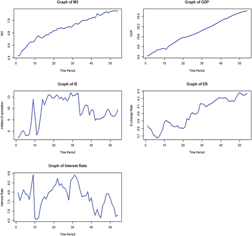
Table 3. Descriptive statistics

Variables	Min	Max	1.Qu.	3.Qu.	Mean	Median	Stdev	Skew	Kurt
LnM3	6.427	7.157	6.749	7.041	6.883	6.890	0.200	−0.448	−0.718
LnY	9.618	10.507	9.855	10.324	10.083	10.074	0.269	−0.026	−1.274
${\pi }^e$	4.800	12.800	8.250	11.700	9.565	9.700	2.369	−0.464	−0.922
LnER	3.675	4.278	3.829	4.173	4.009	4.018	0.188	−0.194	−1.475
r	6.539	8.927	7.402	8.184	7.767	7.833	0.632	−0.221	−0.718

Notes: Min stands for minimum, Max for maximum, 1.Qu. is the first quartile, 3.Qu. is the third quartile, Stdev is the standard deviation, Skew stands for skewness, and Kurt depicts kurtosis.

Source: Authors’ calculation

Table 4. Unit root test results

Variables	ADF Statistics				PP Statistics
	Level	p-Value	First Diff	p-Value	Level	p-Value	First Diff	p-Value
LnM3	3.591	0.99	−2.484	0.01	4.665	1.00	−5.651	0.00
LnY	−2.153	0.50	−6.689	0.00	−2.555	0.30	−6.697	0.00
${\pi }^e$	−2.467	0.34	−7.705	0.00	−2.022	0.58	−7.610	0.00
LnER	−2.723	0.23	−5.418	0.00	−3.040	0.13	−5.420	0.00
r	−2.614	0.09	-	-	−2.690	0.08	-	-

Notes: First diff and p-Value stand for first difference and probability value, respectively

Source: Authors’ calculation

Table 5. Results of bounds test for cointegration, diagnostic testing, and parameter stability test

Panel A: Bounds testing result
Test Statistics	Value		K
F-statistic	3.95		4
Critical bounds values
	10%		5%			1%
Bounds	I(0)	I(1)	I(0)		I(1)	I(0) 4.244	I(1)
F-statistic	2.578	3.710		3.068	4.334		5.726
Panel B: Series of diagnostic testing
Diagnostic test	Jarque-Bera	Breusch-Pagan/Cook-Weisberg				Breush-Godfrey		Ramsey RESET
Statistic	2.154		0.980			14.454		1.780
p-value	0.34		0.32			0.00		0.17
Panel C: Parameters Stability Test
Method	Test Statistic		Critical Values
			10%			5%		1%
Recursive	0.370		0.850			0.948		1.143
OLS	0.360		1.224			1.358		1.628

Notes: RESET stands for regression specification error test.

Source: Authors’ calculation

Figure 2. Plot of recursive CUSUM.

Source: Authors’ calculation

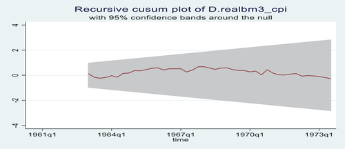
Figure 3. Plot of OLS CUSUM.

Source: Authors’ calculation

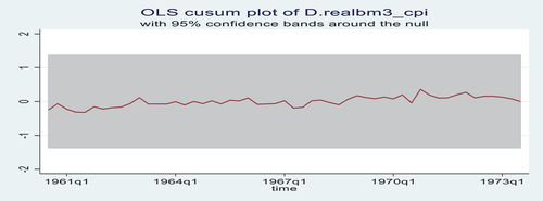
Table 6. Dynamically simulated ARDL results

Variables	Coefficients	SE	t-statistic	p-value
Panel A: Short-run coefficients
ΔLnYt	0.092	0.248	0.370	0.71
Δ rt	0.004	0.006	0.560	0.58
Δ${\pi }^e$t	−0.005	0.003	−2.060	0.05
ΔLnERt	0.037	0.069	0.530	0.60
ECTt-1	−0.234	0.088	−2.650	0.01
Panel B: Long-run coefficients
LnM3t-1	−0.811	0.158	−5.130	0.00
LnYt-1	0.202	0.087	2.330	0.03
rt-1	0.005	0.006	0.730	0.47
${\pi }^e$t-1	−0.008	0.003	−3.130	0.00
LnERt-1	0.027	0.070	0.390	0.70
Adj. R-squared	0.533	Simulations	5000
F-statistic p-value	0.00	Observations	50

Note: All abbreviations are defined in Table 2

Source: Authors’ calculation

Figure 4. The impulse response plot for GDP.

Note: This figure shows one standard deviation positive shock in GDP and its impact on M3. The dots show the mean change in the predicted value from the sample mean. The shaded area shows (from darkest blue to lightest blue) the 75%, 90%, and 95% confidence intervals.

Source: Authors’ calculation

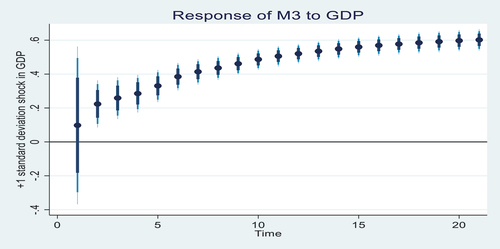
Figure 5. The impulse response plot for GDP.

Note: This figure shows one standard deviation negative shock in GDP and its impact on M3. The dots show the mean change in predicted value from the sample mean. The shaded area shows (from darkest blue to lightest blue) the 75%, 90%, and 95% confidence intervals.

Source: Authors’ calculation

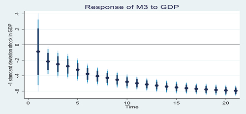
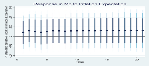
Figure 6. The impulse response plot for inflation expectation.

Note: This figure shows one standard deviation positive shock in inflation expectation and its impact on M3. The dots show the mean change in the predicted value from the sample mean. The shaded area shows (from darkest blue to lightest blue) the 75%, 90%, and 95% confidence intervals.

Source: Authors’ calculation

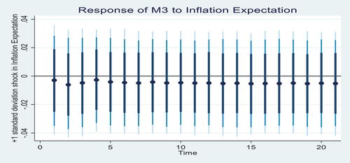
Figure 7. The impulse response plot for inflation expectation.

Note: This figure shows one standard deviation negative shock in inflation expectation and its impact on M3. The dots show the mean change in predicted value from the sample mean. The shaded area shows (from darkest blue to lightest blue) the 75%, 90%, and 95% confidence intervals.

Source: Authors’ calculation

Moosa, I. A. (1992). The demand for money in India: A cointegration approach. The Indian Economic Journal, 40(1), 101. https://doi.org/10.1177/0019466219920106

 Google Scholar

Arrau, P., & De Gregorio, J. (1993). Financial innovation and money demand: Application to Chile and Mexico. The Review of Economics and Statistics, 75(3), 524–530. https://doi.org/10.2307/2109469

 Web of Science ®Google Scholar

Dekle, R., & Pradhan, M. (1999). Financial liberalization and money demand in the ASEAN countries. International Journal of Finance & Economics, 4(3), 205–215. https://doi.org/10.1002/(SICI)1099-1158(199907)4:3<205:AID-IJFE107>3.0.CO;2-G

 Web of Science ®Google Scholar

Funke, N., & Thornton, J. (1999). The demand for money in Italy, 1861–1988. Applied Economics Letters, 6(5), 299–301. https://doi.org/10.1080/135048599353276

 Web of Science ®Google Scholar

Ball, L. (2001). Another look at long-run money demand. Journal of Monetary Economics, 47(1), 31–44. https://doi.org/10.1016/S0304-3932(00)00043-X

 Web of Science ®Google Scholar

Bahmani-Oskooee, M., & Ng, R. C. W. (2002). Long-run demand for money in Hong Kong: An application of the ARDL model. International Journal of Business and Economics, 1(2), 147.

 Google Scholar

Payne, J. E. (2003). Post stabilization estimates of money demand in Croatia: Error correction model using the bounds testing approach. Applied Economics, 35(16), 1723–1727. https://doi.org/10.1080/0003684032000152871

 Web of Science ®Google Scholar

Ramachandran, M. (2004). Do broad money, output, and prices stand for a stable relationship in India? Journal of Policy Modeling, 26(8–9), 983–1001. https://doi.org/10.1016/j.jpolmod.2004.08.008

 Web of Science ®Google Scholar

James, G. A. (2005). Money demand and financial liberalization in Indonesia. Journal of Asian Economics, 16(5), 817–829. https://doi.org/10.1016/j.asieco.2005.08.003

 Google Scholar

Ball, L. (2012). Short-run money demand. Journal of Monetary Economics, 59(7), 622–633. https://doi.org/10.1016/j.jmoneco.2012.09.004

 Web of Science ®Google Scholar

Bahmani-Oskooee, M., Bahmani, S., Kones, A., & Kutan, A. M. (2015). Policy uncertainty and the demand for money in the United Kingdom. Applied Economics, 47(11), 1151–1157. https://doi.org/10.1080/00036846.2014.993138

 Web of Science ®Google Scholar

Belongia, M. T., & Ireland, P. N. (2019). The demand for Divisia Money: Theory and evidence. Journal of Macroeconomics, 61, 103128. https://doi.org/10.1016/j.jmacro.2019.103128

 Web of Science ®Google Scholar

Adil, M. H., Haider, S., & Hatekar, N. R. (2020a). Empirical Assessment of Money Demand Stability Under India’s Open Economy: Non-linear ARDL Approach. Journal of Quantitative Economics, 18(4), 891–20. https://doi.org/10.1007/s40953-020-00203-1

 Google Scholar

De La Fuente, G. G., De La Horra, L. P., & Perote, J. (2020). The demand for Divisia money in the United States: Evidence from the CFS Divisia M3 aggregate. Applied Economics Letters, 27(1), 41–45. https://doi.org/10.1080/13504851.2019.1606403

 Web of Science ®Google Scholar

Barnett, W. A., Ghosh, T., & Adil, M. H. (2022). Is money demand really unstable? Evidence from Divisia monetary aggregates. Economic Analysis & Policy, 74, 606–622. https://doi.org/10.1016/j.eap.2022.03.019

 Web of Science ®Google Scholar