Linear Transport in Porous Media

Figures & data

Table A1. The dependence of $n(L,t)/n_0$ on K for N = 30, $k_{\text{max}}=40,$ M = 40.

$K\backslash t$	$5\text{min}$	$10\text{min}$	$15\text{min}$	$20\text{min}$
0.6	−0.0451	2.77	3.59	3.79
1	1.36	3.72	4.39	4.52
2	1.38	3.73	4.39	4.53
6	1.38	3.73	4.39	4.53
10	1.38	3.73	4.39	4.53
20	1.37	3.74	4.39	4.52
30	1.49	3.71	4.33	4.52
60	3.88	4.12	3.62	3.26

Table A2. The dependence of $n(L,t)/n_0$ on N for K = 6, $k_{\text{max}}=40,$ M = 40.

$N\backslash t$	$5\text{min}$	$10\text{min}$	$15\text{min}$	$20\text{min}$
5	1.65	4.35	5.09	5.23
10	1.33	3.64	4.30	4.44
15	1.38	3.74	4.41	4.54
20	1.38	3.74	4.40	4.53
25	1.38	3.73	4.40	4.53
30	1.38	3.73	4.39	4.53
35	1.38	3.73	4.39	4.53

Figure 1. The particle number density is plotted as a function of t. The blue curve is from (4.3) and the red curve is from (4.4).

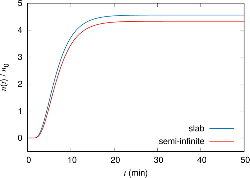
Table A3. The dependence of $n(L,t)/n_0$ on $k_{\text{max}}$ for K = 6, N = 30, M = 40.

$k_{\text{max}}$\t	$5\text{min}$	$10\text{min}$	$15\text{min}$	$20\text{min}$
10	−0.40	2.43	3.30	3.51
20	1.38	3.73	4.39	4.53
30	1.38	3.73	4.39	4.53
40	1.38	3.73	4.39	4.53
50	1.38	3.73	4.39	4.53

Table A4. The dependence of $n(L,t)/n_0$ on M for K = 6, N = 30, $k_{\text{max}}=40.$

M\t	$5\text{min}$	$10\text{min}$	$15\text{min}$	$20\text{min}$
30	1.38	3.73	4.39	4.53
40	1.38	3.73	4.39	4.53
50	1.38	3.73	4.39	4.53
60	1.38	3.73	4.39	4.53

Figure 2. The breakthrough curve of $C/C_0$ (Left) and $1-C/C_0$ (Right) as a function of time. The experimental data (black open circles) are compared with numerical values computed from (4.3) and (4.4) using the linear transport equation in the slab geometry (blue dashed line) and half-space geometry (red line).

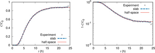
Table 1. Fitted parameters.

	σs (${\mathrm{h}}^{-1}$)	v0 ($\text{cm}/\mathrm{h}$)	u ($\text{cm}/\mathrm{h}$)	β
slab	1.98	3.31	1.52	0.25
half space	2.68	4.12	1.80	0.21