Modified Fokker-Planck Acceleration for Forward-Peaked Transport Problems in Slab Geometry

Figures & data

Figure 1. MFPA algorithm.

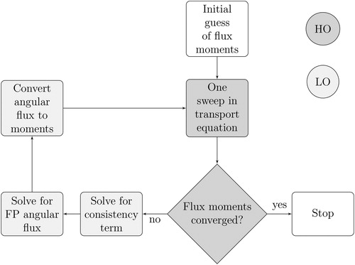
Table 1. Problem parameters.

	Problem set 1	Problem set 2
Q(x)	0.5	0
ψL	0	$\delta (\mu -{\mu }_N)$
ψR	0	0

Figure 2. Screened Rutherford Kernels.

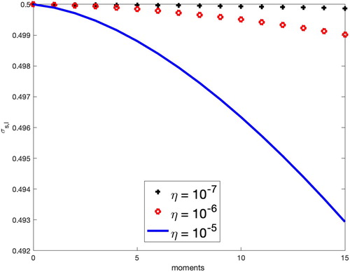
Figure 3. Results for SRK problems with $\eta ={10}^{-7}.$

Table 2. Runtime and iteration counts for Problem 1 with SRK.

Parameter	Solver	Runtime (s)	Iterations
$\eta ={10}^{-5}$	DSA	2380	53,585
	FPSA	1.21	26
	MFPA	1.39	26
$\eta ={10}^{-6}$	DSA	3040	69,156
	FPSA	0.747	16
	MFPA	0.857	16
$\eta ={10}^{-7}$	DSA	3270	73,940
	FPSA	0.475	10
	MFPA	0.542	10

Table 3. Runtime and iteration counts for Problem 2 with SRK.

Parameter	Solver	Runtime (s)	Iterations
$\eta ={10}^{-5}$	DSA	1107	25,072
	FPSA	0.953	20
	MFPA	1.14	20
$\eta ={10}^{-6}$	DSA	1434	32,562
	FPSA	0.730	14
	MFPA	0.857	14
$\eta ={10}^{-7}$	DSA	1470	33,246
	FPSA	0.438	8
	MFPA	0.484	8

Figure 4. Log scale of % relative error vs. η for Problem 1 at the center of the slab with SRK.

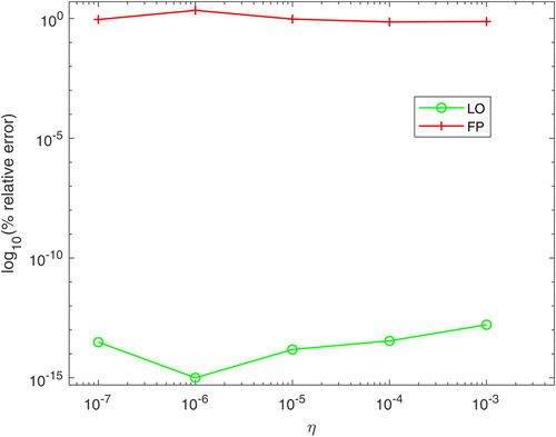
Table 4. Runtime and iteration counts for Problem 1 with SRK.

Parameter	Solver	Runtime (s)	Iterations
$\eta ={10}^{-5}$	GMRES	143	2210
	FPSA-GMRES	0.589	11
	MFPA-Picard	1.02	18
	MFPA-GMRES	0.539	11
$\eta ={10}^{-6}$	GMRES	216	3780
	FPSA-GMRES	0.367	6
	MFPA-Picard	0.558	10
	MFPA-GMRES	0.399	7
$\eta ={10}^{-7}$	GMRES	168	3600
	FPSA-GMRES	0.274	6
	MFPA-Picard	0.301	5
	MFPA-GMRES	0.311	4

Table 5. Runtime and iteration counts for Problem 2 with SRK.

Parameter	Solver	Runtime (s)	Iterations
$\eta ={10}^{-5}$	GMRES	62.6	810
	FPSA-GMRES	0.608	11
	MFPA-Picard	0.664	12
	MFPA-GMRES	0.517	10
$\eta ={10}^{-6}$	GMRES	107	72
	FPSA-GMRES	0.432	7
	MFPA-Picard	0.347	6
	MFPA-GMRES	0.389	7
$\eta ={10}^{-7}$	GMRES	113	1458
	FPSA-GMRES	0.309	4
	MFPA-Picard	0.237	4
	MFPA-GMRES	0.357	4

Figure 5. Exponential Kernels.

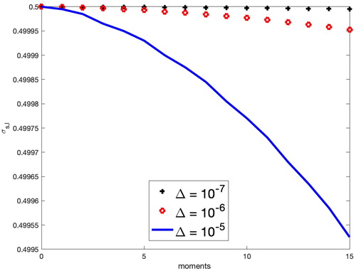
Figure 6. Results for EK Problems with $\Delta ={10}^{-7}.$

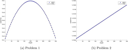
Table 6. Runtime and iteration counts for Problem 1 with EK.

Parameter	Solver	Runtime (s)	Iterations
$\Delta ={10}^{-5}$	DSA	3110	70,140
	FPSA	0.514	11
	MFPA	0.630	11
$\Delta ={10}^{-6}$	DSA	3120	70,758
	FPSA	0.388	7
	MFPA	0.393	7
$\Delta ={10}^{-7}$	DSA	3120	70,851
	FPSA	0.292	6
	MFPA	0.318	6

Table 7. Runtime and iteration counts for Problem 2 with EK.

Parameter	Solver	Runtime (s)	Iterations
$\Delta ={10}^{-5}$	DSA	1455	33,033
	FPSA	0.492	10
	MFPA	0.613	10
$\Delta ={10}^{-6}$	DSA	1470	33,309
	FPSA	0.358	7
	MFPA	0.431	7
$\Delta ={10}^{-7}$	DSA	1470	33,339
	FPSA	0.273	5
	MFPA	0.319	5

Table 8. Runtime and iteration counts for Problem 1 with EK.

Parameter	Solver	Runtime (s)	Iterations
$\Delta ={10}^{-5}$	GMRES	206	4140
	FPSA-GMRES	0.320	5
	MFPA-Picard	0.350	6
	MFPA-GMRES	0.298	5
$\Delta ={10}^{-6}$	GMRES	143	2860
	FPSA-GMRES	0.237	3
	MFPA-Picard	0.240	4
	MFPA-GMRES	0.228	3
$\Delta ={10}^{-7}$	GMRES	124	486
	FPSA-GMRES	0.228	3
	MFPA-Picard	0.185	3
	MFPA-GMRES	0.226	3

Table 9. Runtime and iteration counts for Problem 2 with EK.

Parameter	Solver	Runtime (s)	Iterations
$\Delta ={10}^{-5}$	GMRES	96.0	544
	FPSA-GMRES	0.324	5
	MFPA-Picard	0.257	4
	MFPA-GMRES	0.293	5
$\Delta ={10}^{-6}$	GMRES	80.1	533
	FPSA-GMRES	0.236	3
	MFPA-Picard	0.183	3
	MFPA-GMRES	0.226	3
$\Delta ={10}^{-7}$	GMRES	62.8	1110
	FPSA-GMRES	0.237	3
	MFPA-Picard	0.126	2
	MFPA-GMRES	0.182	2

Figure 7. Henyey–Greenstein Kernels.

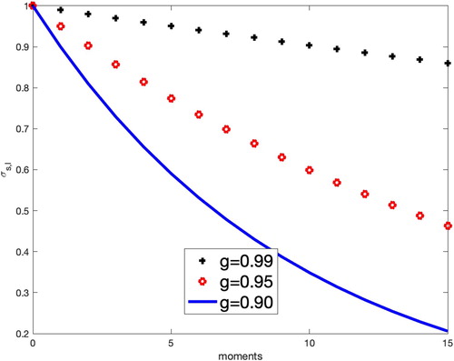
Figure 8. Results for HGK Problems with g = 0.99.

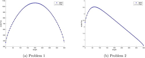
Table 10. Runtime and iteration counts for Problem 1 with HGK.

Parameter	Solver	Runtime (s)	Iterations
g = 0.9	DSA	24.5	554
	FPSA	1.50	32
	MFPA	1.39	27
g = 0.95	DSA	47.7	1083
	FPSA	1.75	38
	MFPA	1.83	35
g = 0.99	DSA	243	5530
	FPSA	3.38	74
	MFPA	3.93	73

Table 11. Runtime and iteration counts for Problem 2 with HGK.

Parameter	Solver	Runtime (s)	Iterations
g = 0.9	DSA	14.8	336
	FPSA	1.15	23
	MFPA	1.35	24
g = 0.95	DSA	29.7	675
	FPSA	1.56	32
	MFPA	1.90	33
g = 0.99	DSA	146	3345
	FPSA	3.31	67
	MFPA	3.99	67

Table 12. Runtime and iteration counts for Problem 1 with HGK.

Parameter	Solver	Runtime (s)	Iterations
g = 0.9	GMRES	98.6	92
	FPSA-GMRES	0.494	9
	MFPA-Picard	1.24	21
	MFPA-GMRES	0.512	10
g = 0.95	GMRES	106	2112
	FPSA-GMRES	0.618	12
	MFPA-Picard	1.63	29
	MFPA-GMRES	0.632	13
g = 0.99	GMRES	85.7	1131
	FPSA-GMRES	1.161	24
	MFPA-Picard	3.13	58
	MFPA-GMRES	1.135	26

Table 13. Runtime and iteration counts for Problem 2 with HGK.

Parameter	Solver	Runtime (s)	Iterations
g = 0.9	GMRES	29.1	265
	FPSA-GMRES	0.678	13
	MFPA-Picard	1.07	19
	MFPA-GMRES	0.659	14
g = 0.95	GMRES	36.9	330
	FPSA-GMRES	0.864	17
	MFPA-Picard	1.46	26
	MFPA-GMRES	0.863	19
g = 0.99	GMRES	39.9	14
	FPSA-GMRES	1.53	32
	MFPA-Picard	2.98	54
	MFPA-GMRES	1.49	35

Figure 9. Results for heterogeneous Problem 1 using SRK with $ϵ=\pm 0.4,\pm 0.8.$

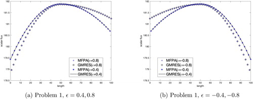
Figure 10. Results for heterogeneous Problem 2 using SRK with $ϵ=\pm 0.4,\pm 0.8.$

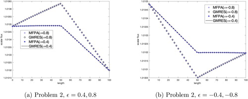
Figure 11. Results for heterogeneous Problem 1 using EK with $ϵ=\pm 0.4,\pm 0.8.$

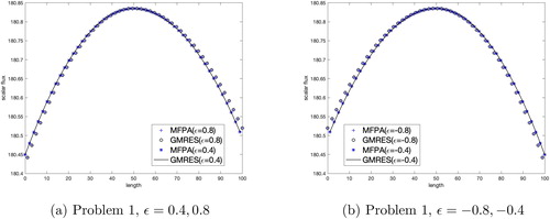
Figure 12. Results for heterogeneous Problem 2 using EK with $ϵ=\pm 0.4,\pm 0.8.$

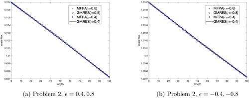
Figure 13. Results for heterogeneous Problem 1 using HGK with $ϵ=\pm 0.4,\pm 0.8.$

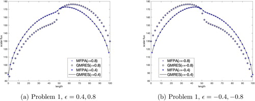
Figure 14. Results for heterogeneous Problem 2 using HGK with $ϵ=\pm 0.4,\pm 0.8.$

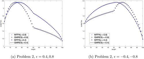
Table 14. Theoretical spectral radius results for MFPA.

Kernel	Parameter	ρth	ρnu
SRK	$\eta ={10}^{-7}$	0.298	0.299
EK	$\Delta ={10}^{-7}$	0.114	0.110
HGK	g = 0.99	0.760	0.759

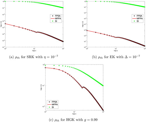
Figure 15. Results of ρ_th for SRK, EK, and HGK.