Development and evaluation of a method to define a tibial coordinate system through the fitting of geometric primitives

Figures & data

Table 1. Definitions of coordinate system for the knee

OT	The X-coordinate equal to half the distance between the most medial and lateral points of the distal femur, Y-coordinate equal to the point of intersection between the longitudinal axis and the XTYT plane containing the most inferior point of the medial femoral condyle and the Z-coordinate equal to the most inferior point of the medial femoral condyle.
XT	The axis of the cone fitted to the posterior distal condyles of the femur
YT	Cross-product between XT and ZT
ZT	Longitudinal axis of tibia determined through cone fit using tibial shaft

Figure 1. Workflow for development of coordinate system. A – longitudinal axis of tibia workflow. Ai – cone fit applied to full length tibia from proximal joint to distal joint establishing reference axis. Aii – user-selected slice made below tibial tuberosity along with computer generated slice 200 mm below initial slice, cone fit to be applied between two slices. Aiii – cone fit applied between two slices with axis established through center of cone. proximal and distal aspects of tibia discarded showing only section of tibia to which the cone fit is applied. the axis is represented as the blue line. Aiv – Successive discarding of 10 mm of tibial shaft to test application of cone at each changing shaft length. B – mediolateral axis of tibia workflow. Bi – reconstructed distal femur with automated slices made to isolate posterior aspect of femoral condyles (highlighted in red). Bii – sagittal slice made to outer aspect of each condyle isolating a condylar width of 12 mm. Biii – cone fit applied to initial condylar width showing direction of mediolateral axis. the axis is represented as the red line. C – coordinate system generation. longitudinal axis of tibia, Z_T (blue), mediolateral axis of femur, X_T (red) and orthogonal axis, Y_T (green). Ci – anterior view. Cii – lateral view

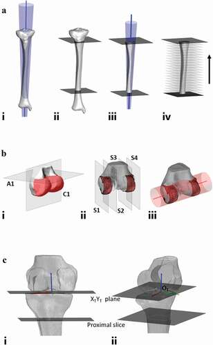
Figure 2. Mean error of the longitudinal axis angles within the coronal and sagittal planes from the angle measured using the entire tibia. A – coronal plane. B – sagittal plane. shaded error bars represent the standard deviation of the axis angle. the dashed line represents the point at which the angular deviation is considered too great and thus any application of the cone fit should be at lengths greater than this point

Figure 3. Bland-Altman plots comparing the difference for the two angles and the limits of agreement. A – coronal plane. B – sagittal plane. only shaft lengths of 50 mm or greater are presented due to the noted variability at shorter lengths. UL, upper limit; LL, lower limit

Table 2. Mean error of the mediolateral axis angles within the coronal and axial planes, against that measured using automated identification of the outermost medial and lateral points of the femur

	Condylar Width (mm)
Planar Angle	12	9	6	3
Coronal (°)	2.59 ± 1.88	2.68 ± 1.93	2.68 ± 1.93	2.43 ± 2.01
Axial (°)	2.72 ± 2.11	2.87 ± 1.95	3.10 ± 2.09	3.31 ± 2.24

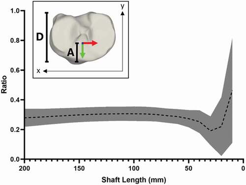
Figure 4. Mean position of Y-coordinate for origin at varying shaft lengths, based on ratio of anterior depth to tibial plateau depth. inset; method for determining the ratio, the distance from the most anterior point of the articular surface to the position of the origin along the Y axis (A) against the total tibial plateau depth determined as the distance between the outermost anterior and posterior points of the articular surface (D).