Figures & data
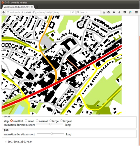
Figure 1. Example of how to obtain content for a Space-Scale Cube (SSC): ➀ from a sequence of generalization operations, ➁ a Directed Acyclic Graph (DAG) can be derived and ➂ the DAG and step-wise generalization results can be converted in a 3D data cube, the SSC. In this example, the colours blue, grey, yellow and green respectively represent water, road, farmland and forest terrains.
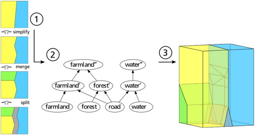
Figure 2. A 2D map from the SSC can be obtained by slicing: calculating the resulting intersection of the 3D cube with a 2D surface.
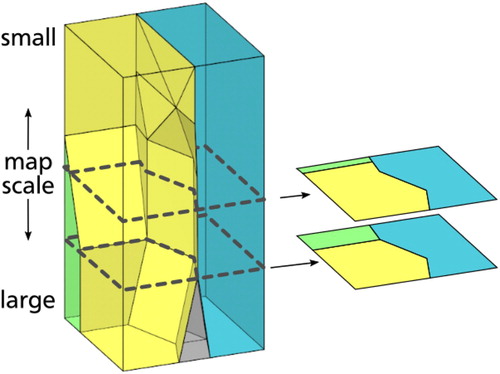
Figure 3. Comparing vertical with tilted trans-scale boundaries. (a) Vertical trans-scale boundaries between grey area object on the left and white area object on the right. Note that the grey object has a horizontal top (at which it disappears from the map). (b) Maps obtained by slicing at 4 different locations in the cube. Slices as viewed from the top. Outcome of merge appears at once. (c) Tilted trans-scale boundaries describe how the grey area object on the left is merged gradually to the white area object on the right. (d) Maps obtained by slicing at 4 different locations in the cube. Slices as viewed from the top. Outcome of merge is presented gradually to the end user.
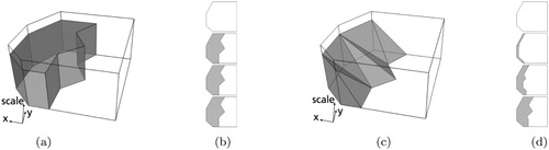
Figure 4. When a polyline is simplified, the outcome of the simplification can be stored as trans-scale boundary. (a) A trans-scale boundary for a polyline simplified with the Visvalingham-Whyatt algorithm (the original polyline is visualized with the black line at the bottom of the trans-scale boundary). Each time a vertex is removed from the polyline, this results in a triangle in the resulting transscale boundary. (b) Slicing at different locations through the resulting trans-scale boundary, leads to a polyline with less (top) or more (bottom) vertices. Result of slicing operation shown in perspective view.
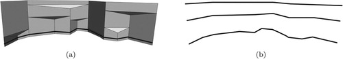
Figure 5. The rendering approach its goal is to determine what ‘colour’ to give each pixel in a raster. To do this, the centre points of the pixels are tested for what colour polyhedron it is inside. This example highlights a single row of grid points in the raster, and determines that in this row, 1 pixel shows forest, 4 shows farmland and 3 shows water. Because of the placement of the points, the road is not visible. (a) Raster placement viewed where the plane is intersecting. (b) Raster placement in 3D. (c) Side view on one row of pixels, represented as their centers.
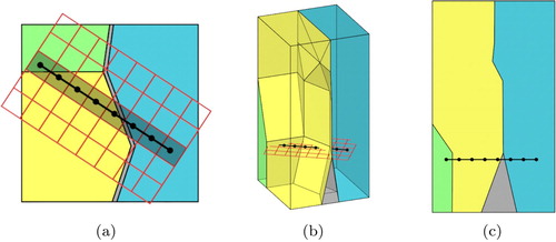
Figure 6. By shooting a ray through the grid points downwards we find the correct colours for the pixels. The greyed area must be explicitly ignored, otherwise some invalid colours will appear. In this example, if the greyed region was not clipped the first and fifth pixels would incorrectly get assigned yellow and blue respectively.
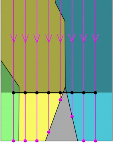
Figure 7. Intersecting an SSC in real time. SSC data runs through some steps on the GPU (the rendering pipeline) before a map is displayed to the end user. Note that the steps in green are programmable and can be modified by the programmer. Image after Hock-Chuan (Citation2019).
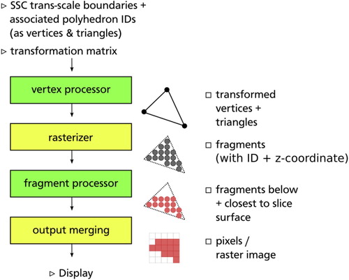
Figure 8. In this example, the centre of the raster requires less abstraction than the raster edges. As a result, the forest becomes invisible and the road visible.
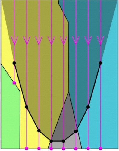
Figure 9. The three marked points represent an intersection within the given distance. The left and middle points will blend yellow-green and yellow-grey respectively. The right point resides on the cube boundary, so blending will not occur there.
Figure 10. This example shows how a transition from one object (a) to the next (d) can be abrupt while zooming out (the purple object at the bottom takes over the region of the yellow object in the middle). This is noticeable, while the slicing surface is in motion, zooming in or out. Compared to (b) when near-blending is disabled (c) blending the colours makes the transition appear less abrupt.
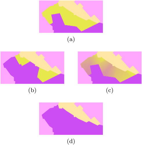
Figure 11. Texturing is shown as the numbers rendered in the regions. They fade on the sides because of the non-planar intersection used to generate the image, showing that abstraction variations influence the result.

Figure 12. Architecture overview. How data flows through the architecture for each map image to be rendered is shown.
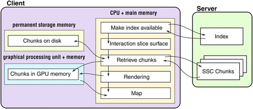
Figure 13. Protocol for retrieving (a) tGAP data compared to (b) SSC data.
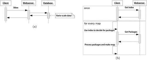
Figure 14. Testing data based on the SSC model, shown at the highest level of detail. (a) Land cover dataset (source: CORINE Land Cover dataset, Middlesbrough, UK). (b) City centre dataset (source: TOP10NL, Leiden city centre, NL). (c) Rural region dataset (source: TOP10NL, near Maastricht, NL).
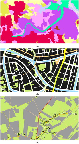
Figure 15. The slice surface on the left produces the corresponding map image shown on the right. Note that with higher level of detail more buildings and roads become visible. (a) Horizontal slice plane. (b) Map scale equal everywhere. (c) Sine curve slice plane. (d) Larger map scale in the middle.
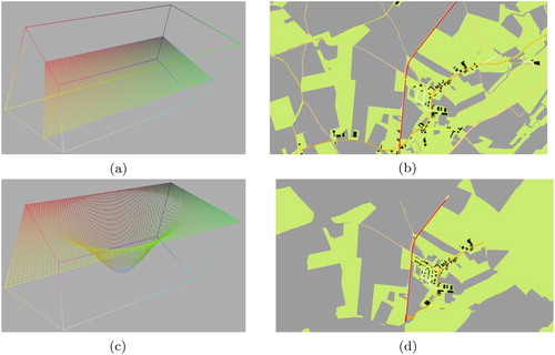
Figure 16. Parameters for controlling smooth transitions as implemented in the user interface.