Figures & data
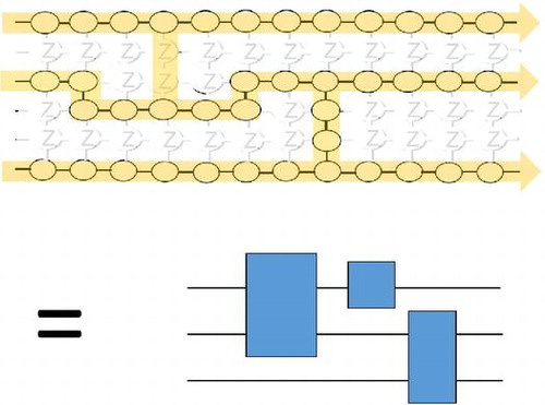
Figure 1. Gate teleportation: (a) a single one, (b) cascade of (a) four times.
Figure 2. Conversion of graph states: (a) Square lattice; (b) Brickwork lattice. Solid black circles indicate Z measurements and meshed red circles indicate Y measurement.
Figure 3. Gates implementation: (a) two independent one-qubit gates; (b) CNOT gate. The symbols inside the circles indicate the measurement angles.
Figure 4. From AKLT to a graph state. (a) A spin-1 chain; (b) Spin-3/2 case on the honeycomb lattice. Encoding is indicated by shapes with the same color. The new edges are derived from the original edges in a mod-2 fashion, as can be seen in (b).
Figure 5. AKLT states on graphs or 2D lattices. (a) Arbitrary graph: showing virtual qubits on each site. The physical spin is a projection from the symmetric subspace of the virtual qubits to a spin S Hilbert space. (b) Honeycomb lattice. (c) Square-octagon lattice. (d) Cross lattice. (e) Hexagon-square lattice. (f) Square lattice.
Figure 6. Fixed-point SPT states: (a) on the square lattice; (b) on the honeycomb lattice.
Figure 7. Entanglement concentration: converting the SPT state to a known universal resource state.
Figure 8. (a) Triangular lattice; (b) Union-Jack Lattice.