Figures & data
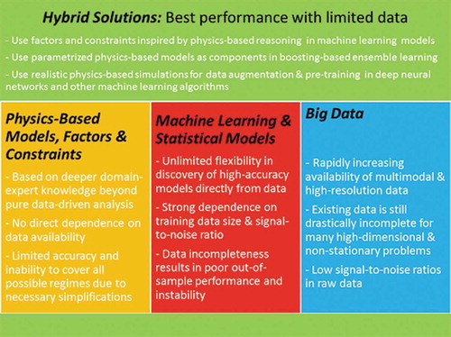
Figure 1. Schematic of a typical neuron-like computational unit used in NN architectures. Each neuron can receive inputs from one or many other neurons via connections, known as synapses. If the sum of all inputs becomes larger than a certain threshold, a neuron fires (i.e. the neuron sends a signal to other neurons to which it is connected). In general, this process is controlled by nonlinear activation, described by a transfer function, where sigmoid (left panel) and/or rectified linear (right panel) functions are often used in practice.
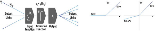
Figure 4. Schematic of the recurrent neural network (RNN) with several feedback loops. Unlike MLP, RNN can have feedback loops in different parts of the NN structure, including feedbacks skipping one or more layers. RNN can build robust models of complex sequential data using implicit representation in its internal memory. However, training based on a Back-propagation Trough Time (BPTT) algorithm could often encounter vanishing- or exploding-gradient problems in practice.
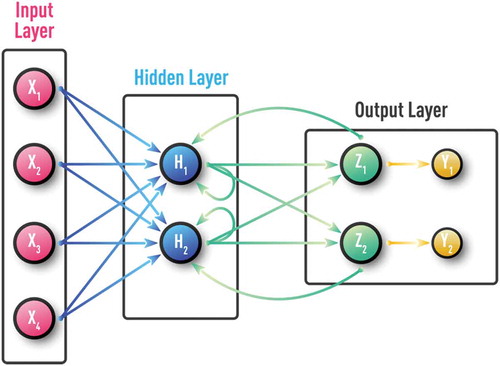
Figure 2. Schematic of unsupervised Kohonen NN or self-organizing map (SOM) with 1D (left panel) and 2D (right panel) architectures. These NNs are trained by competitive unsupervised learning algorithms and used for clustering of unlabeled data and discovery of low-dimensional representations.
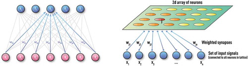
Figure 6. Schematic of classical gradient descent in 1D (left panel) and stochastic gradient descent (SGD) in 2D (right panel) which is used in NN training with error back-propagation algorithm.
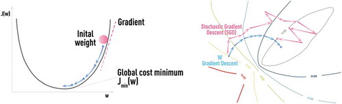
Figure 7. Schematic of saddle point with vanishing gradients. Stochasticity, naturally introduced in SGD by considering errors from only part of training samples at a time, helps escaping saddle points which presents a real obstacle for regular gradient descent methods suffering from vanishing gradients.
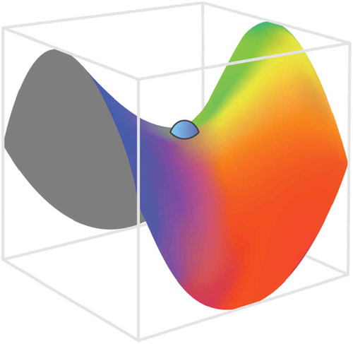
Figure 8. Problems of sub-optimal learning rate (large and small). Finding the optimal SGD parameters that avoid such problems, as ‘trap in local minima’ or ‘very noisy and slow convergence (if any)’, could be challenging and application-dependent without any single universal solution.
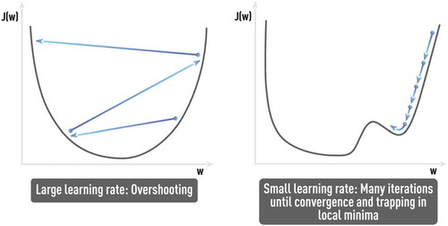
Figure 9. Schematic of bias-variance tradeoff. Generic behavior of model error computed on test and training samples for different degrees of model complexity. The model error on the training set will continue decreasing with increasing model complexity. However, the minimum testing error is achieved at some optimal value of model complexity.
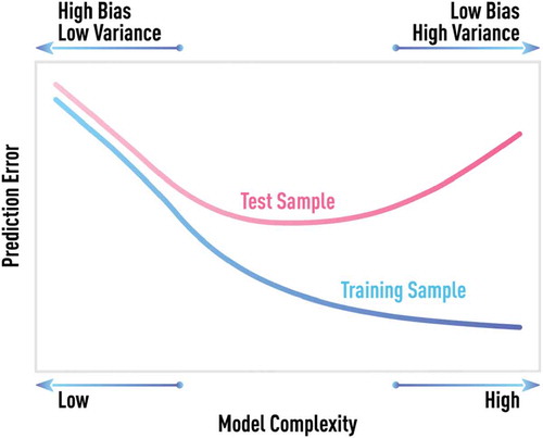
Figure 10. Schematic of optimal model selection using the principle of structural risk minimization (SRM). SRM fits a nested sequence of models of increasing VC dimensions h1 < h2 < … < hn and then chooses the model with the smallest value of the upper-bound estimate. Algorithms (like SVM) that are based on the SRM principle incorporate regularization that is aimed at better out-of-sample performance, into the training procedure itself.
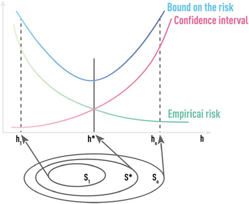
Figure 11. Schematic of larger margin classifier (a), compared to smaller margin classifier (b). Support vectors (dashed lines) define boundaries of the classes and the decision hyperplane (solid line) is specified to be equidistant from the two support vectors. SVM algorithm, based on the SRM principle, can find the optimal support vectors and the corresponding decision boundary to ensure large separation (i.e. large margin) between classes, ensuring good out-of-sample performance.
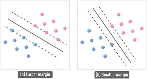
Figure 12. Schematic of quadratic dependence estimation from a very limited data set with and without domain knowledge about the estimated function. Available noisy data (red circles) for the unknown quadratic function y = ax2 (blue line) cover a very limited range. It is impossible to choose the correct complexity of the fitting model (for extrapolation) without incorporating any additional information. Most statistical algorithms would choose linear regression (orange line) with bad out-of-sample performance. However, if domain knowledge hints to quadratic nature of the functional form, estimating the parameter a in y = ax2 from a few available data points leads to low-complexity model (grey line) with very good out-of-sample performance.
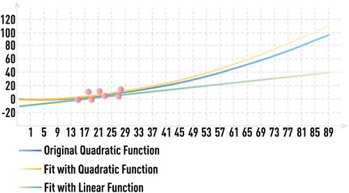
Figure 13. Schematics of a generic boosting algorithm with decision stump (i.e. one-level decision tree) as a base model. Such generic, application-independent, base model is a typical choice in pure data-driven approaches.
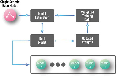
Figure 14. Schematics of boosting algorithm with multiple well-understood and low-complexity domain-expert models as base models. Such a procedure can test and utilize the complementary value of any number of available domain-expert models without overfitting. Proper parameterization could also allow discovery of many complementary models, even from a single domain-expert model.
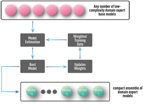
Figure 15. Schematics of DNN with stacked auto-encoders followed by supervised NN. First, the auto-encoder layers are trained in unsupervised fashion using labeled and unlabeled data. Then, the MLP classifier is trained on labeled data using usual supervised learning, while weights from the first set of layers are kept constant. For further reduction of requirement on training data size, single multi-layer auto-encoder is replaced by a stack of shallow auto-encoders (e.g. each with only one hidden layer) that are trained one at a time.
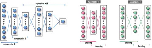
Figure 3. Schematic of a supervised feed-forward neural network also known as multi-layer perceptron (MLP). MLP is a feed-forward NN with at least one hidden layer and supervised training procedure, which is usually based on an error back-propagation (BP) algorithm. MLP can be effective for capturing complex patterns in both regression and classification problems.
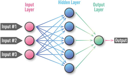
Figure 16. Schematic of representation by similarity. Novel class (llama) is represented as a vector of probabilities of three well-known classes (giraffe, sheep, and dog) to which a novel example belongs.

Figure 17. Schematic of classical boosting-based ensemble learning and ensemble decomposition learning (EDL) based on the boosting ensemble. The EDL vector provides universal and fine-grain representation not only for the two learned classes but also for sub-classes/sub-states within these two classes.
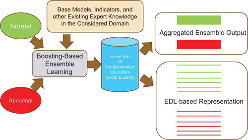
Figure 18. Schematic of ECG waveform and its main elements: the P wave representing the depolarization of the atria, the QRS complex representing the depolarization of the ventricles, the T wave representing the repolarization of the ventricles and others. Inter-beat interval signal (R-R time series) can be extracted with high accuracy even from noisy ECG waveform recordings.
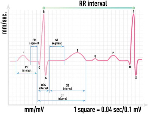
Figure 5. Schematic of error surfaces of low (left panel) and high (right panel) complexity corresponding to problems of low and high dimensionality, respectively. The error function in the high-dimensional space becomes more complex with increasing number of hard-to-avoid local minima.
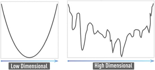
Figure 19. Detection (i.e. true positive) rates of CHF, LTAF, and arrhythmia for different false alarm (i.e. false positive) rates. All presented measures are computed on short RR segments of 256 beats which is relevant for express diagnostics or monitoring when only a short-duration ECG time series is available. Ensemble-based indicator shows significant improvement over single measures in all three cases of different abnormalities.
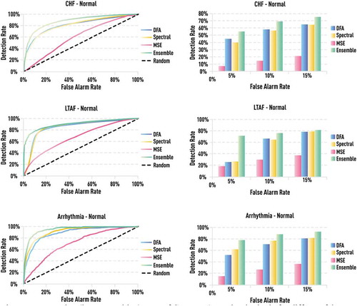
Figure 20. Receiver operating characteristic (ROC) curves of the ensemble indicator. Left: ROC curves of the aggregated ensemble-based indicator. Right: ROC curves based on EDL metrics of the same indicator using full ensemble (green) and MSE-only subset (dashed green). EDL-based ROC curve is significantly better than that based on the aggregated value. By choosing certain sub-components of the ensemble (e.g. only MSE), one can further improve differentiation based on EDL metrics.
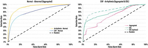
Figure 21. MST-based distances between each pair of 20 CHF patients using a collection of 50 consecutive EDL vectors computed on 256-beat RR segments. For each subject, distances to all other subjects are represented by black circles. Distance to his own portion of RR time series, not overlapping with the original one, is shown by a red circle. Distance of the subject to himself is either minimal or close to minimal.
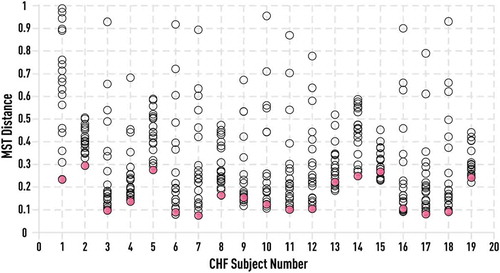
Figure 22. Rank of the MST-based distance of each healthy, CHF, and LTAF subject to himself against distances to other subjects within the same group. Rank 1 corresponds to minimal distance. Ensemble-based rank (green) is compared to those based on single measures: DFA (blue) and LFHF (yellow). Ensemble-based measure provides a significantly more accurate ranking compared to any single measure.
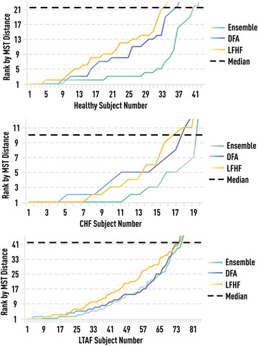
Figure 23. Schematic diagram of the cardiovascular/respiratory model proposed in [Citation58]. The diversity in the model is caused mainly by factors such as time delays in the neural conduction, multiplications in neural and mechanical variables, and time-varying Windkessel dynamics. The model consists of a system of delay-differential equations.
![Figure 23. Schematic diagram of the cardiovascular/respiratory model proposed in [Citation58]. The diversity in the model is caused mainly by factors such as time delays in the neural conduction, multiplications in neural and mechanical variables, and time-varying Windkessel dynamics. The model consists of a system of delay-differential equations.](/cms/asset/7ad87229-7b4f-45c5-a9b1-72b22b7312ea/tapx_a_1582361_f0023_oc.jpg)
Figure 24. Single DFA measure computed on each of 128-interval segments of stride data from the normal control group and patient groups with ALS, HD, and PD (left panel). Aggregated ensemble measure computed on each of 128-interval segments of stride data from the normal control group and patient groups with ALS, HD, and PD (right panel). Although the best single indicator computed on short gait time series is still capable to provide some differentiation between normal and abnormal states, boosting-based combination significantly improves such differentiation.
Figure 25. Abnormality detection rates for a given false alarm rate: The best single measure vs ensemble of multi-complexity measures. Although the best single indicator computed on short gait time series is still capable to provide some differentiation between normal and abnormal states, boosting-based combination drastically increases the detection rate (by 40–50%) for reasonable false alarm rates.
Figure 26. 10-th percentile of the distribution of ensemble (left panel) and single indicators (two right panels) computed on the consecutive 256-beat RR segments of 1 hour Holter monitor recordings before (green) and during (blue) Chi meditation for 7 subjects. Ensemble-based measure clearly shows the expected improvement of the psychophysiological state in meditation compared to the pre-meditation period. Although single measures also indicate the correct direction, there is significant overlapping between pre-meditation and meditation states.
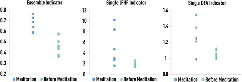
Figure 27. Single DFA measure computed on each of 128-interval segments of stride data from three different age groups of healthy subjects (upper panel). Aggregated ensemble measure computed on each of 128-interval segments of stride data from three different age groups of healthy subjects (bottom panel). A single DFA indicator is not capable to detect any clear trend in gait dynamics with respect to the short-intervals evolution as child age increases, while the multi-complexity ensemble indicator shows a clear trend towards gait dynamics of healthy adults as age increases.