Optical Emission Spectroscopic (OES) analysis for diagnostics of electron density and temperature in non-equilibrium argon plasma based on collisional-radiative model

Figures & data

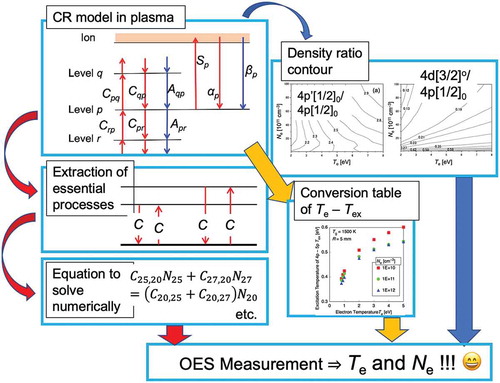
Figure 1. Schematic diagram of excitation kinetics of the level p in the collisional-radiative (CR) model. Red arrows indicate electron collisional processes, while the blue arrows indicate radiative processes. Characters in the figure correspond to their rate coefficients in Equation (1).

Figure 2. Schematic diagram of the ‘phases’ of the hydrogen-like ionizing plasma; i.e. ‘Corona phase’, ‘Saturation (Thermodynamically Equilibrium: TE) phase’ and ‘Saturation (Ladder-like) phase’. p is the principal quantum number, N/g is the reduced population density. The straight arrow indicates electron collision excitation/deexcitation process, while the wavy arrow indicates radiative process. Horizontal axis denotes the logarithm of reduced electron density divided by z ⁷. The phase transition lines ‘GRIEM’ and ‘BYRON’ indicate the Griem’s boundary (Equation (5)) and the Byron’s boundary (Equation (6)), respectively [33,37].

Figure 3. Essential elementary processes for the population and depopulation of the level N = 20 (4d + 6s) for the electron temperature range (a) 0.8 ≤ T_e [eV] ≤ 1.2 and (b) 1.2 ≤ T_e [eV] ≤ 2.0. The symbol C denotes the electron collision process. It is found that C_23,30N₂₃$\simeq$C_20,23N₂₀ under the condition (a), and consequently, the equation to be solved can be simplified.

Figure 4. Comparison of the electron temperature measured with the Langmuir probe and that with the OES method assisted with the CR model described by Equations (11) – (14) as schematically shown in Figure 3 for the hollow cathode DC discharge argon plasma for its discharge current 6 A [72].

Figure 5. Density contour of number density ratio of the excited states calculated with the argon CR model, displayed on T_e-N_e map. (a) 4p’ [1/2]₀/4p[1/2]₀, and (b) 4d[3/2]°/4p[1/2]₀ [44].

Figure 6. Electron temperature and density measured for the argon plasma generated in the small helicon device (SHD) developed for the electric propulsion of satellite maneuver [81–83]. Red open squares are those measured with the scheme described in section 3.2, with two intensity ratios of (687.1 nm)/(763.5 nm) [= 4d[1/2]°/4p[3/2] = 4d₅/2p₆] and (549.6 nm)/(751.5 nm) [= 6d[7/2]°/4p[1/2]₀ = 6d’₄/2p₅] with most revised cross section data in Ref [78]., while green open diamonds are the same but with the old cross section data in Ref [40]. Blue filled dots are those measured with a Langmuir single probe.

Figure 7. Reduced number densities N/g of the levels 4p, 4p’, 5p and 5p’, calculated with the argon CR model normalized by that of the 4p[1/2]₁ level. Linear fitting in the figure gives the excitation temperature with its slope. When the fitting is conducted, the statistical weight is reflected for the regression calculation.

Figure 8. The relationship between the electron temperature T_e and the excitation temperature T^ex determined for 4p – 5p levels calculated with the argon CR model. It is assumed that the gas temperature T_g = 1500 K and the discharge tube radius R = 5 mm, with the electron density N_e = 10¹⁰–10¹² cm^–3 [87,88].

Fujimoto T. Plasma Spectroscopy. Oxford: Clarendon Press; 2004.

 Google Scholar

Fujimoto T. Kinetics of ionization-recombination of a plasma and population density of excited ions. IV. Recombining plasma–low-temperature case. J Phys Soc Jpn. 1980;49:1569.

 Google Scholar

Kano K, Suzuki M, Akatsuka H. Spectroscopic measurement of electron temperature and density in argon plasmas based on collisional-radiative model. Plasma Sources Sci Technol. 2000;9:314.

 Web of Science ®Google Scholar

Bogaerts A, Gijbels R, Vlček J. Collisional-radiative model for an argon glow discharge. J Appl Phys. 1998;84:121.

 Web of Science ®Google Scholar

Kuwahara D, Mishio A, Nakagawa T, et al. Development of very small-diameter, inductively coupled magnetized plasma device. Rev Sci Instrum. 2013;84:103502.

 PubMed Web of Science ®Google Scholar

Nakagawa T, Sato Y, Tanaka E, et al. Study on magnetized RF discharge with very small-diameter. Plasma Fusion Res. 2015;10:3401037.

 Google Scholar

Keesee AM, Scime EE. Neutral argon density profile determination by comparison of spectroscopic measurements and a collisional-radiative model (invited). Rev Sci Instrum. 2006;77:10F304.

 Web of Science ®Google Scholar

Vlček J. A collisional-radiative model applicable to argon discharges over a wide range of conditions. I. Formulation and basic data. J Phys D Appl Phys. 1989;22:623.

 Web of Science ®Google Scholar

Akatsuka H, Yuji T, Fujioka K, et al. Estimation of electron temperature of non-equilibrium argon plasma of atmospheric pressure by OES measurement. Proc 24th Symp Plasma Proc. Osaka, Japan: 2007;24:387.

 Google Scholar

Akatsuka H, Yuji T, Urayama T, et al. Estimation of electron temperature of non-equilibrium argon plasma of atmospheric pressure by OES measurement. Proc. 3rd Int. Con. Cold Atm. Press. Plasma Sources Appl. (CAPPSA-3); Gent, Belgium: 2007. p.1.

 Google Scholar