Engineered electronic states in atomically precise artificial lattices and graphene nanoribbons

Figures & data

Figure 1. (a-e) Lattice structures and the Brillouin zones of the honeycomb (a), kagome (b) and Lieb (d) lattices. (f-h) Corresponding band structures calculated with the nearest-neighbour tight-binding model for the honeycomb (f), kagome (g) and Lieb (h) lattices. (i) The Lieb lattice band structure when second nearest-neighbour hoppings are introduced ($t^{\prime }=0.2t$). The energies have been scaled by the nearest neighbour hopping strength $t$.

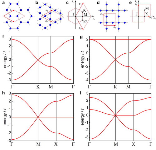
Figure 2. Experiments on artificial graphene. (a) Cu(111) surface state electrons are patterned by CO molecules ordered through STM lateral manipulation. (b) d$I$/d$V$ spectroscopy reveals the appearance of a Dirac cone in the band structure in the patterned area. (c) The effect of strain can be mimicked by continuously modulating the lattice spacing of the artificial graphene. The effective pseudomagnetic field strengths are indicated in the panels. (d) d$I$/d$V$ spectroscopy shows the formation of Landau levels due to the pseudomagnetic field generated by strain. Adapted by permission from Springer Nature: Ref. 11, Copyright (2012).

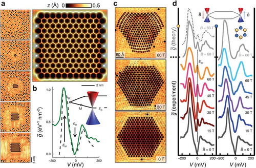
Figure 3. Experiments on artificial lattices. (a,b) Lieb lattice made with CO molecules on Cu(111) substrate (a) and the corresponding density of states measured on the different lattice sites within the unit cell (b). Adapted by permission from Springer Nature: Ref. 52, Copyright (2017). (c-e) Sierpiński triangle fractal lattice constructed using CO on Cu(111) (c) and the corresponding measurement of the fractal dimension (d) and estimation of the fractal dimensions of the LDOS as a function of the energy of the G(3) Sierpiński triangle (orange) and comparison with the 2D square lattice (blue) for the experimental (dark) and muffin-tin (light) wavefunction maps (e). Adapted by permission from Springer Nature: Ref. 53, Copyright (2019). (f) Lieb lattice constructed from chlorine vacancies on the c$(2\times 2)$ chlorine structure on Cu(100) and the corresponding measured (middle) and calculated LDOS (bottom) maps at the energy corresponding to the flat band position. Adapted by permission from Springer Nature: Ref. 65, Copyright (2017). (g) Different artificial lattices with engineered band structures constructed using the chlorine vacancy system. Adapted by permission from SciPost: Ref. 84, Copyright (2017).

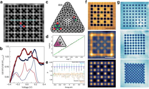
Figure 4. (a) The two phases in the SSH model where the strong hopping is either inside the unit cell (phase A) or between the unit cells (phase B). (b) Structure containing a domain wall where the intra-unit-cell ($t_1$) and inter-unit-cell $t_2$ hoppings are inverted. (c) Plots of $\mathbf{d}(k)\hat{\sigma }=d_x{\hat{\sigma }}_x+d_y{\hat{\sigma }}_y$ as a function of the $\delta t=(t_1-t_2)/2$. The red circle marks the transition between the topological and trivial phases with the associated closing of the gap. (d) Experimental realization of a structure with two domain walls using the Cl vacancy system (top) and the corresponding experimental (middle) and calculated (bottom) LDOS maps of the domain wall states. Adapted by permission from Springer Nature: Ref. 65, Copyright (2017).

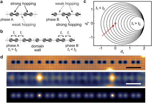
Figure 5. Nanoribbon synthesis and properties. (a) Schematic of AGNRs and ZGNRs. Adapted by permission from Springer Nature: Ref. 26, Copyright (2016). (b) Schematic of the Ullmann coupling route to synthesize AGNRs. (c-g) Examples of AFM images of (c) 7-AGNR (Adapted by permission from Springer Nature: Ref. 28, Copyright (2013)), (d) ZGNR (Adapted by permission from Springer Nature: Ref. 26, Copyright (2016)), (e) chevron GNRs (here with nitrogen edge doping [103], Adapted by permission from John Wiley and Sons: Ref. 147, Copyright (2016)), (f) boron doped 7-AGNR (Adapted by permission from Springer Nature: Ref. 140, Copyright (2015)) and (g) chiral (3,1)-GNR (Adapted with permission from Ref. 130. Copyright (2017) American Chemical Society). (h-i) Calculated gaps of (h) the different families of armchair GNRs (LDA level of theory) with the corresponding band structures of 13- and 14-AGNRs and (i) the ZGNRs (LDA level of theory) with the corresponding band spin density and band-structure for 12-ZGNR. Adapted with permission from Ref. 114. Copyright (2006) by the American Physical Society.

Figure 6. Experiments on GNR heterostructures. (a) A type 2 heterojunction: pristine (left) and nitrogen-doped (right) chevron-type AGNR heterostructure and the LDOS across it. Adapted by permission from Springer Nature: Ref. 30, Copyright (2014). (b) A type 1 heterojunction: 7–13 AGNR heterostructure. Adapted by permission from Springer Nature: Ref. 31, Copyright (2015). (c,d) A metal-semiconductor junction: 5–7 AGNR heterostructure. d$I$/d$V$ spectra and LDOS maps acquired on a 5–7-5 AGNR heterostructure (c). $I-Z$ and $I-V$ curves obtained while lifting the 5–7-5 AGNR heterostructure (d). Since the ultra-narrow 5-AGNR is nearly metallic [32], the 5–7 AGNR heterostructure resembles a tunnelling barrier in a metallic lead. Adapted by permission from Springer Nature: Ref. 151, Copyright (2016).

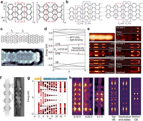
Figure 7. Theory and experiments on topological states in GNRs. (a) Different unit cells in AGNRs give rise to different topological indices. Adapted with permission from Ref. 159. Copyright (2017) by the American Physical Society. (b) Depending on the junction geometry, the topological index can change resulting in the formation of topological domain wall states. Adapted by permission from Springer Nature: Ref. 86, Copyright (2018). (c-e) Topological states in a 7–9 AGNR superlattice. The chemical structure and high-resolution STM image (c), the calculated band structure (d) and the LDOS maps of a 7–9 AGNR superlattice (e). Adapted by permission from Springer Nature: Ref. 86, Copyright (2018). (f-h) Topological states in in-line edge-extended AGNR heterostructure superlattices. The chemical structure and nc-AFM image (f), the calculated band structure (g) and the LDOS maps of an in-line edge-extended AGNR heterostructure superlattice (h). Adapted by permission from Springer Nature: Ref. 87, Copyright (2018).

Durr RA, Haberer D, Lee Y-L, et al. Orbitally matched edge-doping in graphene nanoribbons. J Am Chem Soc. 2018;140:807–813.

 PubMed Web of Science ®Google Scholar

Kimouche A, Ervasti MM, Drost R, et al. Ultra-narrow metallic armchair graphene nanoribbons. Nat Commun. 2015;6:10177.

 PubMed Web of Science ®Google Scholar