
Figures & data
Figure 1. Typical Machine Learning Workflow. Data generated from simulation trajectories is first represented by selecting certain features, usually reducing the dimensionality. Data is then chosen for training the ML tasks to generate a model, which is optimized for its hyperparameters, validated, and tested for overfitting.
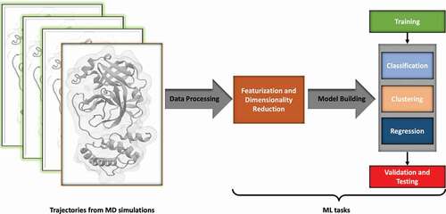
Figure 2. Dimensionality Reduction with Machine Learning. A. PCA is used to detect directions of highest variance. In a two-dimensional case, PCA resolves the variance into two orthogonal Principal Components (PCs). B. Typical eigenvalue spectrum obtained from PCA. PCA can be used to reduce dimensionality by selecting a cut-off, where the variance starts to go asymptotically to zero. C. Comparison of PCA and tICA methods on a two-well potential. Left: Projection of the first PC and tIC on the data. The first tiC correctly identifies the two minima in the free energy surface (FES). Right: tIC finds the direction along the two minima in the FES. D. Kernel PCA solves the PCA problem by first applying a non-linear transform on the data that embeds the data into a higher-dimensional space, where a hyperplane can linearly separate the data points which were not linearly separable earlier.
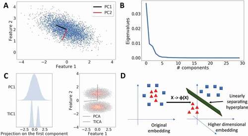
Figure 3. ANNs for Dimensionality Reduction. Autoencoder networks (shown in gray) are used for training a lower-dimensional representation of the simulation data by reconstructing sampled structures (deep blue) with decoded structures (light blue). A trained autoencoder can be used to generate a latent space representation of the data set (blue points), which can used to generate unseen latent space data (red points) to mine unsampled structures (red structures). Figure adapted from Degiacomi et al. [Citation62].
![Figure 3. ANNs for Dimensionality Reduction. Autoencoder networks (shown in gray) are used for training a lower-dimensional representation of the simulation data by reconstructing sampled structures (deep blue) with decoded structures (light blue). A trained autoencoder can be used to generate a latent space representation of the data set (blue points), which can used to generate unseen latent space data (red points) to mine unsampled structures (red structures). Figure adapted from Degiacomi et al. [Citation62].](/cms/asset/ed05830c-34eb-4220-98ec-f8b6cb76d17b/tapx_a_2006080_f0003_oc.jpg)
Figure 4. Principal Component Regression (PCR). A. PCR-based ensemble-weighted mode for the Leucine Binding Protein. B. Coefficient αi of the contribution to the PCR model from the largest PCA eigenvectors. C. Eigenvalues of the PCs used to construct the PCR model. D. Contribution of the variance of the PCs to the variance of the collective mode. Figure adapted from Hub et al. [Citation63].
![Figure 4. Principal Component Regression (PCR). A. PCR-based ensemble-weighted mode for the Leucine Binding Protein. B. Coefficient αi of the contribution to the PCR model from the largest PCA eigenvectors. C. Eigenvalues of the PCs used to construct the PCR model. D. Contribution of the variance of the PCs to the variance of the collective mode. Figure adapted from Hub et al. [Citation63].](/cms/asset/6aec4d28-7d5b-49db-a808-ea3f73cd2fe6/tapx_a_2006080_f0004_oc.jpg)
Figure 5. ANNs for Regression. ANNs can be trained to develop coarse-grained force fields by the force matching method. Physical restrictions of translational and rotational invariance, and conservative forces, are imposed on the regression task performed by the CGnets architecture by a choice of internal coordinates and the GDML layer, whereby the atomistic force field is reduced to a coarse-grained force field. Figure adapted from Wang et al. [Citation71]. Further permissions related to the material excerpted (https://pubs.acs.org/doi/full/10.1021/acscentsci.8b00913) should be directed to the ACS.
![Figure 5. ANNs for Regression. ANNs can be trained to develop coarse-grained force fields by the force matching method. Physical restrictions of translational and rotational invariance, and conservative forces, are imposed on the regression task performed by the CGnets architecture by a choice of internal coordinates and the GDML layer, whereby the atomistic force field is reduced to a coarse-grained force field. Figure adapted from Wang et al. [Citation71]. Further permissions related to the material excerpted (https://pubs.acs.org/doi/full/10.1021/acscentsci.8b00913) should be directed to the ACS.](/cms/asset/465a12ca-099b-414a-91c2-9999883dca44/tapx_a_2006080_f0005_oc.jpg)
Figure 6. Classification and Clustering (Machine Learning) Techniques. A. Partial least squares-based Discriminant Analysis technique (PLS-DA) is used for identifying the collective mode that differentiates between bound and unbound ubiquitin simulations. Projection of the simulation data from the bound and unbound simulations on the difference vector given by the PLS-DA mode separates their distributions. Inset: The structural ensembles of ubiquitin binding region in the unbound and bound mode identified by the PLS-DA eigenvector. Figure adapted from Peters et al. [Citation74]. B. Active and inactive states of the Src kinase are identified from MD simulations with clustering and then classified using a Random Forest (RF) classifier. Using a Gini index, importance is assigned to the residues that contribute most significantly to the classification. Figure adapted from Sultan et al. [Citation76]. Further permissions related to the material excerpted (https://pubs.acs.org/doi/10.1021/ct500353m) should be directed to the ACS. C. L11 · 23S protein-complex is first subjected to dimensionality reduction. The simulation data are projected on the first two eigenvectors and then clustered with the k-means algorithm to identify the structure in the data. Figure adapted from Wolf et al. [Citation35]. D. Gaussian Mixture Model-based clustering is used to identify the free energy minima in Calmodulin simulations using the InfleCS methodology. The GMM is built on a 2D surface using the coordinates reciprocal interatomic distances (DRID) and the linker backbone dihedral angle correlation (BDAC). The most likely transition pathways in these states are identified and plotted on the free energy surface. Figure adapted from Westerlund et al. [Citation96]. Further permissions related to the material excerpted (https://pubs.acs.org/doi/abs/10.1021/acs.jctc.9b00454) should be directed to the ACS.
![Figure 6. Classification and Clustering (Machine Learning) Techniques. A. Partial least squares-based Discriminant Analysis technique (PLS-DA) is used for identifying the collective mode that differentiates between bound and unbound ubiquitin simulations. Projection of the simulation data from the bound and unbound simulations on the difference vector given by the PLS-DA mode separates their distributions. Inset: The structural ensembles of ubiquitin binding region in the unbound and bound mode identified by the PLS-DA eigenvector. Figure adapted from Peters et al. [Citation74]. B. Active and inactive states of the Src kinase are identified from MD simulations with clustering and then classified using a Random Forest (RF) classifier. Using a Gini index, importance is assigned to the residues that contribute most significantly to the classification. Figure adapted from Sultan et al. [Citation76]. Further permissions related to the material excerpted (https://pubs.acs.org/doi/10.1021/ct500353m) should be directed to the ACS. C. L11 · 23S protein-complex is first subjected to dimensionality reduction. The simulation data are projected on the first two eigenvectors and then clustered with the k-means algorithm to identify the structure in the data. Figure adapted from Wolf et al. [Citation35]. D. Gaussian Mixture Model-based clustering is used to identify the free energy minima in Calmodulin simulations using the InfleCS methodology. The GMM is built on a 2D surface using the coordinates reciprocal interatomic distances (DRID) and the linker backbone dihedral angle correlation (BDAC). The most likely transition pathways in these states are identified and plotted on the free energy surface. Figure adapted from Westerlund et al. [Citation96]. Further permissions related to the material excerpted (https://pubs.acs.org/doi/abs/10.1021/acs.jctc.9b00454) should be directed to the ACS.](/cms/asset/b4c97862-38af-461b-a34a-6e9c6db5df72/tapx_a_2006080_f0006_oc.jpg)
Figure 7. ANNs for Classification. ANNs used for classification of GPCRs based on differences in a bound agonist. The geometric coordinates are first encoded into the RGB code to generate a two-dimensional image. Using a convolutional neural network architecture, the map between the image and the corresponding level is learnt. Sensitivity analysis is used to retrace the pixels in the image and then from them the corresponding residues that are mainly responsible for the classification task. Figure adapted from Plante et al. [Citation98].
![Figure 7. ANNs for Classification. ANNs used for classification of GPCRs based on differences in a bound agonist. The geometric coordinates are first encoded into the RGB code to generate a two-dimensional image. Using a convolutional neural network architecture, the map between the image and the corresponding level is learnt. Sensitivity analysis is used to retrace the pixels in the image and then from them the corresponding residues that are mainly responsible for the classification task. Figure adapted from Plante et al. [Citation98].](/cms/asset/fe3b8cef-eca2-4d71-a4fc-1007b9dcd63e/tapx_a_2006080_f0007_oc.jpg)