Strong-field physics with nanospheres

Figures & data

Figure 1. Strong-field physics with atomic targets. (a) Three-step model. An electron can (i) tunnel through the finite barrier of the effective potential (solid black curve), (ii) be accelerated by the laser field (red curve), and (iii) recollide with the ion resulting in elastic backscattering or recombination. (b) HATI spectrum from Ar under 40 fs 630 nm pulses at $I=1.2\times {10}^{14}\mathrm{W}/\mathrm{c}{\mathrm{m}}^2$. Adapted from [16]. (c) Intensities of harmonics of 1064 nm pulses generated in Xe at I ≈ $3\times {10}^{13}\mathrm{W}/\mathrm{c}{\mathrm{m}}^2$. Adapted from [13]. Arrows indicate the spectral cut-offs as predicted by the three-step model. (d) Trajectories for direct emission (black) and with one recollision (red) for different birth times (colored dots). Bold curves reflect optimal trajectories for direct emission ‘1ʹ, elastic backscattering ‘2ʹ and recombination ‘3ʹ. Dashed red and black curves visualize the evolution of laser electric field and its vector potential. White and gray areas indicate quarter-cycles of the field. (e) Birth time-dependent final energies for direct emission (black curve) and backscattering (solid red), and recollision energies (solid blue). Recollision timings are indicated by respective dashed curves. From [45].

Figure 2. Enhanced near-fields at nanostructures. (a) Maximum enhancements of the radial near-fields at small and large silica nanospheres under 5 fs 720 nm few-cycle pulses with respect to the peak field strength of the incident field (Mie calculations). (b) Near-field at a tungsten nanotip with 10 nm apex radius and opening angle $\alpha =15$° under a 5 fs 800 nm few-cycle laser pulse propagating in $z$-direction and polarized in $x$-direction. Gray arrows indicate the local orientation of the field at the instant of maximal enhancement. Adapted from [26].

Figure 3. (a) TEM image of SiO₂ nanospheres with a diameter of 147 nm. (b) Flow diagram for the generation of the nanoparticle aerosol. (c) Working principle of an aerodynamic nanoparticle lens. The trajectories of gas molecules are schematically indicated by the blue dashed lines. The nanoparticle trajectories are shown in red. From [62].

Figure 4. Schematic representation of VMI of strong-field induced ionization processes in isolated nanoparticles. Courtesy of Philipp Rupp.

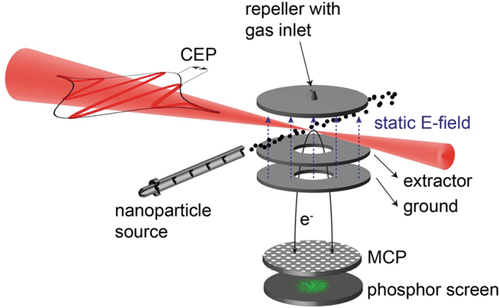
Figure 5. Illustration of efficient background suppression by histogram selection for photoemission from 313 nm SiO₂ nanopspheres under few-cycle laser pulses at 2.7 ×10¹³ W/cm². (a) Histogram of the number of events per frame. (b) Momentum map corresponding to the full histogram selection. (c,d) Momentum maps corresponding to selection of frames with the number of events ranging from 0 to 60 (c) and from 60 to 1000 (d), as indicated by the red and blue areas in (a). Adapted from [62].

Figure 6. Linear response near-fields of nanospheres in quasistatic dipole approximation. (a-c) Absolute value of the near-field in the $y=0$ plane with respect to the field strength of the driving static field ${\mathcal{E}}_0{\mathit{e}}_z$ for three different relative permittivities of the sphere with radius $R$ (as indicated). (d) Field strength along the z axis, i.e. along the dashed vertical lines in (a-c). (e) Maximum enhancement (solid curve) and inside field (dashed curve) in dependence of the materials attenuation factor $\alpha =1/{\epsilon }_{\mathrm{r}}$. Colored dots mark the respective permittivity values of the profiles shown in (d).

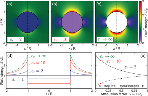
Figure 7. Linear near-field at silica nanospheres. (a) Enhancement of the radial linear near-field at silica spheres (false color plots) with respect to an incident 4 fs few-cycle pulse at 720 nm central wavelength (red curve) in dependence of sphere diameter (respective field propagation parameters $\varrho$ as indicated). The characteristic angles ${\theta }_{\mathrm{h}}$ indicate the hot spots (defined via the maximal enhancement at the surface). Red and blue arrows indicate radial and tangential unit vectors, respectively. Adapted from [45]. (b) Map of the radial surface fields relative enhancement ${\mathcal{E}}_{\mathrm{r}}(d,\theta )/{\mathcal{E}}_0$ with respect to the peak field strength ${\mathcal{E}}_0$ of the incident few-cycle laser pulse, in dependence of the angle $\theta$ sampled at the surface of the upper sphere half in the $z=0$ plane. The white curve indicates the characteristic (hot-spot) angle ${\theta }_{\mathrm{h}}(d)$ of maximum enhancement. (c) Relative enhancements ${\mathcal{E}}_{\mathrm{r}/\mathrm{t}}(d)/{\mathcal{E}}_0$ of the radial (red) and tangential (blue) surface fields, sampled at the characteristic angle. (d) Ellipticity parameter (red) and tilt angle of the local polarization ellipses. Adapted from [46].

Figure 8. Schematic representation of tunneling from the surface of a dielectric. The dashed black curve reflects the effective potential for the atomic case (Coulomb + Laser). Solid red and blue curves represent the effective potentials when considering the enhanced linear (Mie) near-field and the full near-field for an atom located near the surface of a dielectric, respectively. From [45].

Figure 9. Elastic electron-atom scattering in SiO₂. (a) Effective differential cross section in dependence of the incoming electron’s energy $E$ and the scattering angle $\theta$. (b) Energy-dependent effective transport cross section for elastic scattering in SiO₂ (solid red curve). The dashed black and red curves represent the effective molecular transport cross section and a static cross section corresponding to a constant collision frequency, respectively. The horizontal dashed line indicates the geometric cross section of the Wigner-Seitz cell and the vertical dashed line marks the threshold energy, where molecular and geometric cross sections are equal. The solid vertical line marks the effective ionization energy of SiO₂. Transport and total cross section are compared in the top right inset. From [69].

Figure 10. Electron-atom scattering in SiO₂. (a,b) Loss function and inelastic mean free path in dependence of the electrons kinetic energy (blue curves). Adapted from [86] (blue curves) and [88,89,111] (gray curves, as indicated). The gray areas indicate the energy region of interest for the scenarios outlined in this review. (c,d) Energy-dependent elastic and inelastic cross sections (c) and respective scattering times (d). The dashed blue curve in (c) shows the inelastic scattering cross section including all shells of the Si and O atoms. The solid blue curve reflects an effective (scaled) cross section that only includes contributions from the shell with the lowest energy close to the band gap of the SiO₂ nanospheres (for details see [59]) which was sufficient for the theoretical description of most of the considered scenarios. The inelastic scattering time in (d) corresponds to the effective cross section.

Figure 11. Electron emission from silica nanoparticles under intense few-cycle pulses. (a,b) Carrier-envelope phase-averaged maps of the photoelectron momenta in the propagation-polarization (x-y) plane measured (a) from silica nanoparticles (diameter $\approx 100\mathrm{n}\mathrm{m}$) and as predicted by M³C for the experimental parameters (b). The dashed circles indicate the momentum corresponding to an energy of 10 $U_{\mathrm{p}}$. Red and blue shaded areas visualize a 50° full opening angle along the laser polarization axis for upward (red) and downward (blue) emission. Electron kinetic energy spectra are extracted via integration of the data in these regions. (c) CEP-averaged photoelectron energy spectra $Y(E)$ for xenon gas and nanoparticles (as indicated). (d-f) Energy- and CEP-dependent maps of the asymmetry parameter $A=(Y_{\mathrm{u}\mathrm{p}}-Y_{\mathrm{d}\mathrm{o}\mathrm{w}\mathrm{n}})/(Y_{\mathrm{u}\mathrm{p}}+Y_{\mathrm{d}\mathrm{o}\mathrm{w}\mathrm{n}})$, extracted from the electron yields $Y_{\mathrm{u}\mathrm{p}/\mathrm{d}\mathrm{o}\mathrm{w}\mathrm{n}}$ in up- and downward emission direction for silica nanoparticles (d), as predicted by M³C (e) and for xenon gas (f). The limits of the asymmetry color axis in (d), (e) and (f) are set to $\pm 0.4$, $\pm 0.2$ and $\pm 0.6$, respectively. (g) Intensity-dependence of the measured cut-off energies of electrons emitted from $d=(100\pm 50)\mathrm{n}\mathrm{m}$ silica spheres (gray symbols). Solid curves show respective simulation results excluding (black) and including charge interaction (red). Dashed gray and black lines illustrate the classical cut-offs of backscattered electrons for the ponderomotive energies of the incident field $U_{\mathrm{p}}$ and the maximally enhanced local field $U_{\mathrm{p}}^{\mathrm{l}\mathrm{o}\mathrm{c}}={\gamma }_0^2{U}_{\mathrm{p}}$, with peak field enhancement ${\gamma }_0=1.6$. Adapted from [40].

Figure 12. Impact of charge interaction on the electron emission from silica nanospheres (100 nm diameter) under intense few-cycle fields. (a,b) Simulated photoelectron energy spectra of electrons with different numbers of elastic collisions (as indicated) with charge interaction turned off (a) and on (b). The inset in (a) shows the spatial field enhancement profile along the laser fields polarization axis. From [40].

Figure 13. Impact of anisotropic elastic collisions on the electron emission from $d=100\mathrm{n}\mathrm{m}$ SiO₂ nanoparticles under 4 fs NIR few-cycle pulses ($\lambda =720\mathrm{n}\mathrm{m}$, $I=3\times {10}^{13}\mathrm{W}/\mathrm{c}{\mathrm{m}}^2$, ${\phi }_{\mathrm{c}\mathrm{e}}=0$). From [45].

Figure 14. Charge interaction effects in strong-field photoemission from dielectric nanospheres. (a) Evolution of the kinetic energies of typical recollision trajectories corresponding to the cutoff energies of spectra extracted from M³C simulations without (black) and with (red) charge interaction. The cut-offs are defined as the energies where the spectra of single recollision electrons drop by three orders of magnitude (symbols in the inset). Blue and red shaded areas indicate energy gains due to trapping field assisted backscattering (TRAB) and Coulomb explosion of the escaping electron bunch (CE), respectively. (b) Top: Blue plus signs represent positive surface charges from residual ions. Red spheres indicate escaping electrons under the effect of space charge repulsion. Bottom: Attractive trapping potential near the surface mediated by residual ions and emitted electrons (blue) and additional repulsive component (red) due to space-charge repulsion among the escaping electrons. (c) Trajectory analysis of TRAB. Optimal recollision trajectories calculated in the long pulse limit via the conventional SMM (solid black curve) and the SMM extended to account for a triangular trapping potential (solid red curve). The labeled circles mark birth ‘b’, outer turning point ‘t’ and recollision ‘r’ of the respective trajectories. (d) Time evolution of the single particle energies $E_{\mathrm{s}\mathrm{p}}$ corresponding to the respective trajectories in (c). The solid blue curve represents the triangular trapping potential. Vertical dashed gray and blue lines indicate the surface and the end of the trapping potential, respectively. The inset shows the evolution of the single particle energies on a longer timescale. Adapted from [48] and reprinted by permission of Informa UK Limited, trading as Taylor & Francis Group, www.tandfonline.com.

Figure 15. Systematic analysis of trapping field induced quenching and enhancement of the electron emission from surfaces. (a,b) Final energies of optimal trajectories of electrons emitted directly (a) and after elastic backscattering (b) in dependence of the field strength $ϵ$₀ and extension $\alpha$ of a triangular trapping potential. (c) Recollision energies of optimal backscattering trajectories in dependence of the trapping field parameters as in (a) and (b). Insets in (a-c) visualize the respective processes. Dashed black lines in (b) and (c) indicate the optimal parameters for the maximal cut-off and recollision energy, respectively. Adapted from [48] and reprinted by permission of Informa UK Limited, trading as Taylor & Francis Group, www.tandfonline.com.

Figure 16. Quenching the material dependence in strong-field emission from nanospheres. (a-d) Measured cut-off energies of electrons emitted from small (a) SiO₂, (b) ZnS, (c) Fe₃O₄ and (d) PS nanospheres in dependence of the peak intensity at the surface $I_{\mathrm{l}\mathrm{o}\mathrm{c}}$ (symbols) and as predicted by M³C simulations excluding (dashed curves) and including (solid curves) charge interaction. Experimental error bars reflect uncertainties of the laser intensities and in the cut-off evaluation. Gray shaded areas indicate the $10U_{\mathrm{p}}^{\mathrm{l}\mathrm{o}\mathrm{c}}$ cut-off and an energy of $22U_{\mathrm{p}}^{\mathrm{l}\mathrm{o}\mathrm{c}}$. (e) Cut-off energies of photoelectrons from $d=100\mathrm{n}\mathrm{m}$ spheres under few-cycle pulses (5 fs, 720 nm) in dependence of ionization energy and peak intensity of the enhanced linear near-field as predicted by M³C. The vertical line marks the surface field intensity corresponding to a laser intensity of $3\times {10}^{13}\mathrm{W}/\mathrm{c}{\mathrm{m}}^2$ for SiO₂. Horizontal lines indicate the ionization energies of different dielectric nanoparticles (as indicated). Data published in [49], figure adapted from [45].

Figure 17. CEP-averaged projected momentum distributions measured from SiO₂ nanospheres with 95, 313, 400 and 550 nm diameter via velocity map imaging (averaged over millions of laser shots). Note that the intensity of the incident 4 fs NIR (720 nm central wavelength) laser-pulses (red curve in the top left corner) has been adjusted to reach maximal momenta around 2 a.u. for all sphere sizes. The final emission angle ${\theta }_{\mathrm{e}}$ is defined with respect to the pulse propagation direction (x-axis), see 550 nm image. Courtesy of F. Süßmann.

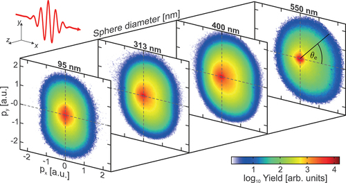
Figure 18. (a,b) CEP-averaged projected momentum maps of electrons emitted from $d=95\mathrm{n}\mathrm{m}$ (a) and 550 nm (b) spheres under 4 fs, 720 nm few-cycle pulses at 3 × 10¹³ W/cm² predicted by M³C. (c) Corresponding CEP-averaged energy spectra (as indicated). Red and blue symbols indicate respective cut-off energies $E_{\mathrm{c}}$, defined as the energy where the yield dropped by three orders of magnitude. (d-g) Directionality and phase-dependent switching. (d,e) Yields $Y({\theta }_{\mathrm{e}},{\phi }_{\mathrm{c}\mathrm{e}})$ of near cut-off electrons (projected momenta $p>\sqrt{2m_{\mathrm{e}}{E}_{\mathrm{t}\mathrm{h}}}$ with threshold energy $E_{\mathrm{t}\mathrm{h}}=0.5E_{\mathrm{c}}$) in dependence of final emission angle ${\theta }_{\mathrm{e}}$ and CEP ${\phi }_{\mathrm{c}\mathrm{e}}$, measured from small (d) and large (e) silica nanospheres. Critical emission angles ${\theta }_{\mathrm{e}}^{\mathrm{c}\mathrm{r}\mathrm{i}\mathrm{t}}$ (vertical dashed lines) and phase offsets $\mathrm{\Delta }\phi ({\theta }_{\mathrm{e}})$ (solid black curves) are defined via the amplitude and phase of harmonic fits of the data for each vertical slice (for details see original publication). The phase offsets at the critical emission angles define the critical phase ${\phi }_{\mathrm{c}\mathrm{e}}^{\mathrm{c}\mathrm{r}\mathrm{i}\mathrm{t}}$ (white symbols). (f,g) M³C predictions for the experimental parameters as in (d,e). Adapted from [45,46].

Figure 19. (a-c) Evolution of measured characteristic emission parameters with sphere diameter (symbols) and respective predictions by SMM (solid black curves) and M³C (solid red curves). (a) Critical emission angles and angles of maximal enhancement of the radial (solid green) and full (dashed green) linear near-fields. (b) Critical phases. (c) Cut-off energies and selective energy gains from different field contributions (as indicated). Shaded areas represent the additional energy gains due to TRAB, CE and tangential field effects. (d,e) Time evolution of the selective kinetic energy gains for two sphere sizes (as indicated). Solid black curves indicate the evolution of the kinetic energies predicted by the SMM. Blue and red curves represent the energy gains from selective contributions to the full near-field (as indicated) for cut-off electrons calculated via M³C (averaged for cut-off electrons). Shaded areas indicate the energy gains from TRAB (blue), Coulomb explosion (red) and tangential field effects (gray). Note the different scaling of the time axes before and after the vertical black lines. Adapted from [45,46].

Figure 20. Photoemission from SiO₂ nanospheres under long pulses. (a,b) Averaged projected momentum maps (in atomic units (a.u.) of momentum) obtained from VMI images of photoelectrons emitted from small (a) and large (b) silica nanospheres under 25 fs laser pulses pulses (central wavelength 780 nm) at 1.32 ×10¹³ W/cm². The color bars represent the electron yields on a logarithmic scale. (c) Open circles show size-dependent $U_{\mathrm{p}}$-rescaled cutoff energies for three different intensities (as indicated, $I_0=8.8\times {10}^{12}\mathrm{W}/\mathrm{c}{\mathrm{m}}^2$). Black squares represent the respective data discussed earlier for few-cycle pulses [46]. Note that the size dependence is expressed via the propagation parameter $\varrho$ to enable comparison with the few-cycle data which was taken at a slightly different wavelength of 720 nm. Adapted from [50].

Figure 21. All-optical directional control of the photoemission from SiO₂ nanospheres in $\omega$-$2\omega$ laser fields. (a) Schematic representation of the enhanced near-field profiles (radial electric field) for the red ($780\mathrm{n}\mathrm{m}$) and blue ($390\mathrm{n}\mathrm{m}$) contributions of a two-color laser field at a $d=300\mathrm{n}\mathrm{m}$ SiO₂ nanosphere. (b-d) Measured angular and relative phase-resolved electron cutoff energies for different sphere diameters and intensity ratios $\eta =I_{2\omega }/I_{\omega }$ (as indicated). The IR intensity was $I_{\omega }=3\times {10}^{12}\mathrm{W}/\mathrm{c}{\mathrm{m}}^2$. Energies are normalized to the ponderomotive potential of the incident IR field. The solid blue lines are angular dependent phase offsets ${\phi }_{\mathrm{o}\mathrm{f}\mathrm{f}\mathrm{s}}({\theta }_{\mathrm{e}})$. Black lines show the relative phase-dependent optimal emission angles ${\theta }_{\mathrm{e}}^{\mathrm{o}\mathrm{p}\mathrm{t}}({\phi }_{\mathrm{r}\mathrm{e}\mathrm{l}})$ of the cutoff energies and white dots indicate the critical emission angles ${\theta }_{\mathrm{e}}^{\mathrm{c}\mathrm{r}\mathrm{i}\mathrm{t}}$. (e-g) Respective maps as predicted by SMM simulations. Adapted from [51] under Creative Commons Attribution 3.0 licence.

Figure 22. (a) Relative phase-dependent optimal emission angles for downward emission obtained from experiment (black) and simulation (blue) with 300 nm SiO₂ nanospheres at $\eta =0.5$ (cf. black curves in Figure 21(d,g)). (b) Intensity ratio-dependent critical emission angles for upward emission obtained from measurement (circles) and SMM simulations (solid blue curve) with 300 nm SiO₂ nanospheres. Adapted from [51] under Creative Commons Attribution 3.0 licence.

Figure 23. (a-i) Recollision-resolved CEP-averaged M³C energy spectra for different sphere diameters and laser intensities (as indicated). Gray shaded areas show full spectra. Solid curves represent selective spectra for direct emission ($n=0$, gray), single recollision ($n=1$, black), and double recollision ($n=2$, red), cf. schematic trajectories in (d). Spectra are normalized to the yield of single recollision electrons at $E=0$. Energies are scaled to the local ponderomotive potential and cut-offs of single and double recollision electrons are indicated as black and red symbols. Dashed vertical lines mark the conventional 10 $U_{\mathrm{p}}^{\mathrm{l}\mathrm{o}\mathrm{c}}$ cut-off. (j,k) Single (black) and double (red) recollision electron yields. (j) Yields in dependence of laser intensity for three nanosphere diameters (as indicated). (k) Yields of all electrons (gray area) and selective yields against nanoparticle diameter for $I=3\times {10}^{13}\mathrm{W}/\mathrm{c}{\mathrm{m}}^2$ (cf. vertical line in (j)). (l,m) Cut-off energies of single and double recollision electrons. (l) Intensity-dependent cutoffs of selective single and double recollision energy spectra and from respective full spectra (dark to light gray areas). (m) Cut-offs against sphere diameter for $I=3\times {10}^{13}\mathrm{W}/\mathrm{c}{\mathrm{m}}^2$ (cf. vertical line in (l)). Adapted from [52].

Figure 24. Trajectory analysis of single and double rescattering. (a) Evolution of radial and tangential excursion with respect to the birth position of typical trajectories extracted for cut-off electrons emitted from 700 nm silica spheres after single (black) and double (red) rescattering. Circles indicate moments of birth ‘b’, first ‘1ʹ and second ‘2ʹ recollision. (b) Evolution of the elliptic local near-fields, sampled along the respective trajectories. (c) Evolution of the velocity components. Jumps at recollisions are indicated as light colored lines. The elliptical features (around$v_r\approx 5$Å/fs) reflect the trivial radial and tangential quiver motions after the recollision phase. The dotted ends of the curves show the additional (mainly radial) velocity gain mediated by the space-charge driven Coulomb explosion of the escaping bunches. Adapted from [52].

Figure 25. Reaction nanoscopy with small and large SiO₂ nanospheres. (a) Schematic setup. Nanospheres and molecular surface adsorbates are ionized by few-cycle laser pulses in the center of the reaction nanoscope. Electrons and ions are recorded in coincidence as fragments arising from molecular photodissociation. Ions are accelerated towards the bottom ion detector (microchannel plates (MCP) and delay-line detector (DLD)) whereas electrons are accelerated towards the opposite side and are detected with a channeltron (top). (b-e) Angle-resolved momentum distributions of emitted protons, obtained via radial integration over the 3D momentum distributions. The number of protons per solid angle is encoded in the color scale. Measured (b) and simulated (c) data for $d=110\mathrm{n}\mathrm{m}$ spheres and (d,e) for $d=300\mathrm{n}\mathrm{m}$ particles, respectively. Adapted from [53].

Figure 26. Subcycle metallization of 95 nm SiO₂ nanospheres under few-cycle NIR laser pulses. (a) CEP-averaged measured electron cutoff energies (black circles) as a function of laser intensity. Blue curves represent cutoffs predicted from M³C simulations for the experimental parameters (including focus averaging) with tunnel ionization enabled only at the surface (dashed) and within the full volume (solid). For the simulations, $\tau =750$ as was considered to mimic the lifetime of plasmonic excitations (cf. Eq. 4(4) ${\sigma }_{\mathrm{e}\mathrm{f}\mathrm{f}}^{\mathrm{t}\mathrm{r}\mathrm{a}\mathrm{n}\mathrm{s}}(\mathrm{E})=\left\{\begin{array}{cc}{\sigma }_{\mathrm{s}\mathrm{t}\mathrm{a}\mathrm{t}}^{\mathrm{t}\mathrm{r}\mathrm{a}\mathrm{n}\mathrm{s}}\left(1-\frac{E}{E_{\mathrm{t}\mathrm{h}}}\right)+{\sigma }_{\mathrm{g}\mathrm{e}\mathrm{o}}\frac{E}{E_{\mathrm{t}\mathrm{h}}}& \mathrm{f}\mathrm{o}\mathrm{r}E\le E_{\mathrm{t}\mathrm{h}}\\ {\sigma }_{\mathrm{e}\mathrm{l}}^{\mathrm{t}\mathrm{r}\mathrm{a}\mathrm{n}\mathrm{s}}& \mathrm{f}\mathrm{o}\mathrm{r}E>E_{\mathrm{t}\mathrm{h}},\end{array}\right.$(4) and respective discussion in the main text). (b) Number density of free electrons $n_{\mathrm{e}}$ at the pulse peak from M³C simulations with and without volume tunneling as function of intensity. The density for which the frequency of the plasmon matches the laser frequency is indicated as resonant density $n_{\mathrm{r}\mathrm{e}\mathrm{s}}$. (c,d) Evolution of the normal component of the internal $\left(x<500\right.$ Å) and external $\left(x>500\right.$Å) near-fields at the surface evaluated along the polarization axis (cf. black arrow in the pictogram in panel (c)) at ${\phi }_{\mathrm{c}\mathrm{e}}=0$ for two different intensities (as indicated). Solid black curves show averaged trajectories of the fastest ten percent of emitted electrons. (e,f) Evolution of the number density of generated electrons from simulations without (dashed) and with (solid) volume tunneling. The red line indicates the electron density at resonance ($n_{\mathrm{r}\mathrm{e}\mathrm{s}}$). (g) Electron density along the x-axis around the upper pole (cf. black arrow in the inset in panel (c)) calculated with volume tunneling for both intensities and averaged during the recollision phase (gray areas in (e) and (f)). Adapted from [69].

Figure 27. Electron cutoff energies measured from different nanoparticles (as indicated) as a function of incident laser intensity. From [69].

Figure 28. Attosecond streaking with dielectric nanospheres. (a) Schematic setup of the experiment. Synchronized attosecond XUV and few-cycle NIR pulses with adjustable delay $\mathrm{\Delta }t$ were shot on a beam of isolated SiO₂ nanopspheres. Emitted electrons were recorded by a single-shot VMI spectrometer. (b,c) Typical single-shot VMI momentum projections recorded from a gas-only measurement (b) and when including silica nanospheres (c) for $\mathrm{\Delta }t=0\mathrm{a}\mathrm{s}$. Dashed circles indicate the low momentum region ($<0.75$ a.u.), where the measured signal contains additional contributions from residual gas background. The gray arrow in (b) illustrates the x-component of the projected momentum of the i-th measured event. Blue and red dots indicate respective averaged projected momenta. (d,e) Respective averaged momentum distributions. Adapted from [59].

Figure 29. Streaking spectrograms and extracted straking delays. (a,b) Attosecond streaking spectrograms obtained from angular integration of projected momentum maps around the laser polarization direction (cf. area indicated in Figure 28(d,e)) for gas (a) and silica nanoparticles (b). To extract the streaking delays energy-dependent frequency-filtered isolines (blue and red dots) were fitted with few-cycle waveforms (blue and red curves) as described in the text. The fits carrier phases define the respective streaking delays $\delta t$. (c) Streaking delays extracted in the high energy range of the measured gas and nanoparticle streaking spectrograms (blue and red dots). Blue and black curves show delays predicted by gas simulations and nanoparticle simulations for the experimental parameters, respectively. The red curve represents the delay extracted from a mixed spectrogram. The dark gray shaded area reflects the maximal variation of the extracted streaking delay when performing the nanosphere simulations with charge interaction enabled or anisotropic elastic collisions. (d) Ratio of nanoparticle to gas signal in dependence of energy extracted from the experiment (red symbols) and from the simulations (black curve). Adapted from [59].

Figure 30. Systematic analysis of the collisional streaking delay calculated via M³C assuming unchirped XUV pulses and energy-independent scattering times to eliminate energy-dependencies of the streaking delays. (a) Streaking delays in dependence of elastic and inelastic scattering times (as indicated). (b) Streaking delays as function of the material’s attenuation factor $\alpha =1/{\epsilon }_{\mathrm{r}}$, where ${\epsilon }_{\mathrm{r}}$ is the relative permittivity at the wavelength of the NIR field. Gray shaded areas in both panels visualize the variation of the streaking delay in dependence of the elastic scattering time. The gray rectangle and the black arrows in (b) indicate permittivities of typical dielectric materials. The dashed black line marks the permittivity of SiO₂. Adapted from [59]. (c) Schematic illustration of attosecond streaking at the surfaces of perfectly transparent (top), typical dielectric (center) and metallic (bottom) targets. After ionization by the XUV pulse (blue) the electron is streaked by the near-field of the optical pulse (red). Adapted from [45].

Paulus GG, Nicklich W, Xu H, et al. Plateau in above threshold ionization spectra. Phys Rev Lett. 1994;72:2851–2854.

 PubMed Web of Science ®Google Scholar

Ferray M, L’Huillier A, Li XF, et al. Multiple-harmonic conversion of 1064 nm radiation in rare gases. J Phys B. 1988;21:L31.

 Web of Science ®Google Scholar

Seiffert L. Semi-classical description of near-field driven attosecond photoemission from nanostructures [dissertation]. University of Rostock; 2018. 10.18453/rosdok_id00002417.

 Google Scholar

Sivis M, Duwe M, Abel B, et al. Nanostructure-enhanced atomic line emission. Nature. 2012;485:E1–E2.

 PubMed Web of Science ®Google Scholar

Süßmann F. Attosecond dynamics of nano-localized fields probed by photoelectron spectroscopy [dissertation]. Ludwig Maximilians University of Munich; 2013. 10.5282/edoc.16144.

 Google Scholar

Süßmann F, Seiffert L, Zherebtsov S, et al. Field propagation-induced directionality of carrier-envelope phase-controlled photoemission from nanospheres. Nat Commun. 2015;6:7944.

 PubMed Web of Science ®Google Scholar

Liu Q, Seiffert L, Süßmann F, et al. Ionization-induced subcycle metallization of nanoparticles in few-cycle pulses. ACS Photonics. 2020;7:3207–3215.

 Web of Science ®Google Scholar

Kuhr JC, Fitting HJ. Monte carlo simulation of electron emission from solids. J Electron Spectrosc Relat Phenom. 1999;105:257–273. 10.1016/S0368-2048(99) 00082–1.

 Google Scholar

Ashley JC, Anderson VE. Energy losses and mean free paths of electrons in silicon dioxide. IEEE Trans Nucl Sci. 1981;28:4131–4136.

 Web of Science ®Google Scholar

Reich T, Yarzhemski VG, Nefedov VI. Calculation of inelastic mean free path of photoelectrons in some solids. J Electron Spectrosc Relat Phenom. 1988;46:255–267.

 Web of Science ®Google Scholar

Tanuma S, Powell CJ, Penn DR. Calculations of electron inelastic mean free paths. iii. data for 15 inorganic compounds over the 50–2000 ev range. Surf Interface Anal. 1991;17:927–939.

 Web of Science ®Google Scholar

Seiffert L, Liu Q, Zherebtsov S, et al. Attosecond chronoscopy of electron scattering in dielectric nanoparticles. Nat Phys. 2017;13:766–770.

 Web of Science ®Google Scholar

Zherebtsov S, Fennel T, Plenge J, et al. Controlled near-field enhanced electron acceleration from dielectric nanospheres with intense few-cycle laser fields. Nat Phys. 2011;7:656–662.

 Web of Science ®Google Scholar

Seiffert L, Henning P, Rupp P, et al. Trapping field assisted backscattering in strong-field photoemission from dielectric nanospheres. J Mod Opt. 2017;64:1096–1103.

 Web of Science ®Google Scholar

Rupp P, Seiffert L, Liu Q, et al. Quenching of material dependence in few-cycle driven electron acceleration from nanoparticles under many-particle charge interaction. J Mod Opt. 2017;64:995–1003.

 Web of Science ®Google Scholar

Powell JA, Summers AM, Liu Q, et al. Interplay of pulse duration, peak intensity, and particle size in laser-driven electron emission from silica nanospheres. Opt Express. 2019;27:27124–27135.

 PubMed Web of Science ®Google Scholar

Liu Q, Zherebtsov S, Seiffert L, et al. All-optical spatio-temporal control of electron emission from SiO2 nanospheres with femtosecond two-color laser fields. New J Phys. 2019;21:073011.

 Web of Science ®Google Scholar

Seiffert L, Süßmann F, Zherebtsov S, et al. Competition of single and double rescattering in the strong-field photoemission from dielectric nanospheres. Appl Phys B. 2016;122:1–9.

 Web of Science ®Google Scholar

Rupp P, Burger C, Kling NG, et al. Few-cycle laser driven reaction nanoscopy on aerosolized silica nanoparticles. Nat Commun. 2019;10:1.

 PubMed Web of Science ®Google Scholar