Magnetoelectricity in two-dimensional materials

Figures & data

Figure 1. Mechanisms underpinning magnetoelectricity in semiconductor-heterostructure quantum wells. Charge carriers can move freely in the $xy$ plane but are confined in $z$ direction by a symmetric potential arising from the spatially varying conduction-band bottom (drawn in black pen). Equilibrium currents [(a)] and bound-state charge distributions [(b)] are indicated in red. The band bending shown schematically in the right panel of subfigure (a) is due to the applied perpendicular electric field. The qualitatively similar, but typically much smaller in magnitude, band bending arising as a consequence of the magnetic-field-induced electric polarization is not shown in the right panel of subfigure (b).

Figure 2. An electric charge $q_0$ placed near a planar interface (located at $z=0$) between an ordinary dielectric (occupying the region $z>0$) and a magnetoelectric medium (present in region $z<0$) generates image dyons on both sides. The values of their electric (magnetic) charges are related via $q_1^{+}=q_1^{-}$ ($g_1^{+}=-g_1^{-}$).

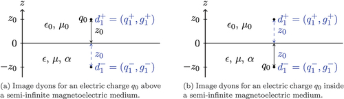
Figure 3. An infinite set of image dyons $d_k^{m\nu }$ is needed to describe electric and magnetic fields generated by an electric point charge $q_0$ placed near [panel (a)] or inside [panel (b)] a finite-width slab of magnetoelectric material. Here $m=\mathrm{U}(\mathrm{L})$ labels dyons arising from mirror-imaging at the upper (lower) boundary, $\nu =+(-)$ when the image dyon is located above (below) the $m$ boundary, and $k\in \mathbb{Z}\mathrm{\setminus }0$ is a counter associated with the dyon location. Dyons with $k<0$ arise only for the case with $q_0$ inside the magnetoelectric medium [panel (b)].

Figure 4. Field lines of the electric ($\mathcal{E}$) and magnetic ($\mathcal{B}$) fields generated by an electric point charge located outside an isotropic magnetoelectric medium occupying the space $0>z>-w$ and having the same dielectric constant and magnetic permeability as the surrounding ordinary medium ($\epsilon ={\epsilon }_0$, $\mu ={\mu }_0$). The black dot indicates the location of the source charge, and horizontal thick blue lines delineate interfaces between ordinary and magnetoelectric media. Green circles are positioned where the interface-current distribution has maxima and show the current direction. Yellow circles are positioned where the interface-charge distribution has maxima and show its sign. The magnetoelectric is assumed to have $\alpha =\sqrt{{\epsilon }_0/{\mu }_0}$.

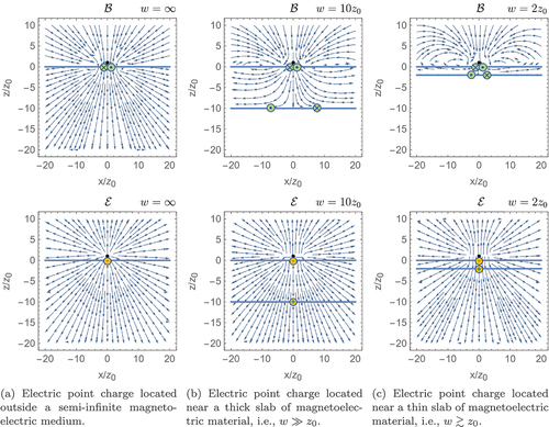
Figure 5. Field lines of the electric ($\mathcal{E}$) and magnetic ($\mathcal{B}$) fields generated by an electric point charge located inside an isotropic magnetoelectric medium occupying the space $0>z>-w$ and having the same dielectric constant and magnetic permeability as the surrounding ordinary medium ($\epsilon ={\epsilon }_0$, $\mu ={\mu }_0$). The black dot indicates the location of the source charge, and horizontal thick blue lines delineate interfaces between ordinary and magnetoelectric media. Green circles are positioned where the interface-current distribution has maxima and show the current direction. Yellow circles are positioned where the interface-charge distribution has maxima and show its sign. The magnetoelectric is assumed to have $\alpha =\sqrt{{\epsilon }_0/{\mu }_0}$.

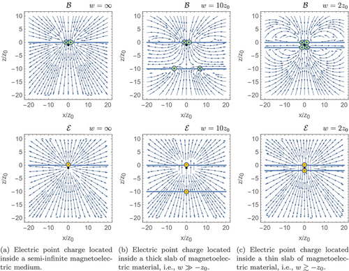
Figure 6. Field lines of the electric ($\mathcal{E}$) and magnetic ($\mathcal{B}$) fields generated by an electric point charge located outside an isotropic magnetoelectric medium occupying the space $0>z>-w$ and having $\epsilon =10{\epsilon }_0$, $\mu ={\mu }_0$, and $\alpha =3\times {10}^{-4}\sqrt{{\epsilon }_0/{\mu }_0}$. The black dot indicates the location of the source charge, and horizontal thick blue lines delineate interfaces between ordinary and magnetoelectric media. Green circles are positioned where the interface-current distribution has maxima and show the current direction. Yellow circles are positioned where the interface-charge distribution has maxima and show its sign.

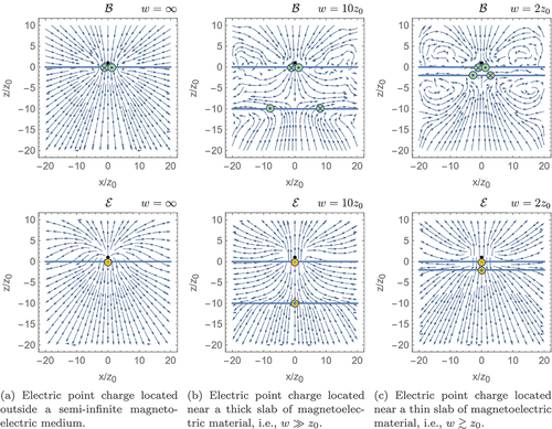
Figure 7. Magnetoelectrically induced interface currents in the slab geometries considered in this work. The blue (yellow) curves show the variation of the current-density component ${\mathcal{J}}_y$ at the upper (lower) boundary as a function of coordinate $x/z_0$. Pairs $(x/z_0,{\mathcal{J}}_y)$ of values associated with positive-current maxima are indicated, allowing also the negative-current maxima to be identified via symmetry as $(-x/z_0,-{\mathcal{J}}_y)$. Panel (a) [(b), (c), (d), (e), (f)] pertains to the situations shown in Figure 4(b) [Figure 6(b), Figure 5(b), Figure 4(c), Figure 6(c), Figure 5(c)].

Table B1. The potentials in terms of image charges when the point charge is above the magnetoelectric slab. Note that $d_1^{\mathrm{L}-}$ does not exist by construction

	Potential	Image charge when ${\epsilon }_0=\epsilon$ and ${\mu }_0=\mu$
$V(R,\theta ,z>0)$	$\frac{1}{4\pi {\epsilon }_0}\left[\frac{q_0}{\left|\mathbf{r}-{\mathbf{r}}_0\right|}+\sum _{m=\mathrm{U},\mathrm{L}}\sum _{k=1}^{\mathrm{\infty }}\frac{q_k^{m-}}{\left|\mathbf{r}-{\mathbf{r}}_k^{-}\right|}\right]$	$q_k^{\mathrm{L}\pm }=0$$q_k^{\mathrm{U}\pm }=\{\begin{array}{cc}-q_0\sigma & k=1\\ q_0\left(1-\sigma \right){\sigma }^{\left(k-1\right)}& k\ge 2\end{array}$
$V(R,\theta ,0>z>-w)$	$\frac{1}{4\pi {\epsilon }_0}\left[\frac{q_0}{\left|\mathbf{r}-{\mathbf{r}}_0\right|}+\sum _{k=1}^{\mathrm{\infty }}\left(\frac{q_k^{\mathrm{U}+}}{\left|\mathbf{r}-{\mathbf{r}}_k^{+}\right|}+\frac{q_k^{\mathrm{L}-}}{\left|\mathbf{r}-{\mathbf{r}}_k^{-}\right|}\right)\right]$
$V(R,\theta ,z<-w)$	$\frac{1}{4\pi {\epsilon }_0}\left[\frac{q_0}{\left|\mathbf{r}-{\mathbf{r}}_0\right|}+\sum _{m=\mathrm{U},\mathrm{L}}\sum _{k=1}^{\mathrm{\infty }}\frac{q_k^{m+}}{\left|\mathbf{r}-{\mathbf{r}}_k^{+}\right|}\right]$
$U(R,\theta ,z>0)$	$\frac{{\mu }_0}{4\pi }\sum _{m=\mathrm{U},\mathrm{L}}\sum _{k=1}^{\mathrm{\infty }}\frac{g_k^{m-}}{|\mathbf{r}-{\mathbf{r}}_k^{-}|}$	$\begin{array}{cc}\hspace{0.17em}& g_k^{\mathrm{U}+}=-g_k^{\mathrm{U}-}\\ =& -g_k^{\mathrm{L}+}=g_{k+1}^{\mathrm{L}-}\\ =& q_0\frac{2\alpha }{4{\epsilon }_0+{\alpha }^2{\mu }_0}{\sigma }^{k-1}\end{array}$
$U(R,\theta ,0>z>-w)$	$\frac{{\mu }_0}{4\pi }\sum _{k=1}^{\mathrm{\infty }}\left(\frac{g_k^{\mathrm{U}+}}{|\mathbf{r}-{\mathbf{r}}_k^{+}|}+\frac{g_k^{\mathrm{L}-}}{|\mathbf{r}-{\mathbf{r}}_k^{-}|}\right)$
$U(R,\theta ,z<-w)$	$\frac{{\mu }_0}{4\pi }\sum _{m=\mathrm{U},\mathrm{L}}\sum _{k=1}^{\mathrm{\infty }}\frac{g_k^{m+}}{|\mathbf{r}-{\mathbf{r}}_k^{+}|}$

Table B2. The potentials in terms of image charges when the point charge is in the magnetoelectric slab. Note that $d_{-1}^{m-}$, $d_{-1}^{\mathrm{U}+}$ and $d_1^{\mathrm{L}-}$ do not exist by construction

	Potential	Image charge when ${\epsilon }_0=\epsilon$ and ${\mu }_0=\mu$
$V(R,\theta ,z>0)$	$\frac{1}{4\pi \epsilon }\left[\frac{q_0}{\left|\mathbf{r}-{\mathbf{r}}_0\right|}+\sum _{m=\mathrm{U},\mathrm{L}}\sum _{k=1}^{\mathrm{\infty }}\frac{q_{\pm k}^{m-}}{\left|\mathbf{r}-{\mathbf{r}}_{\pm k}^{-}\right|}\right]$	$\begin{array}{rl}& q_k^{\mathrm{U}+}=-q_{-(k+1)}^{\mathrm{U}+}\\ & =q_{-k}^{\mathrm{L}+}=-q_k^{\mathrm{L}+}=-q_0{\sigma }^k;\\ & q_{-(k+1)}^{\mathrm{L}-}=-q_{k+1}^{\mathrm{L}-}\\ & =q_k^{\mathrm{U}-}=-q_{-(k+1)}^{\mathrm{U}-}=-q_0{\sigma }^{k-1}\end{array}$
$V(R,\theta ,0>z>-w)$	$\frac{1}{4\pi \epsilon }\left[\frac{q_0}{\left|\mathbf{r}-{\mathbf{r}}_0\right|}+\sum _{k=1}^{\mathrm{\infty }}\left(\frac{q_{\pm k}^{\mathrm{U}+}}{\left|\mathbf{r}-{\mathbf{r}}_{\pm k}^{+}\right|}+\frac{q_{\pm k}^{\mathrm{L}-}}{\left|\mathbf{r}-{\mathbf{r}}_{\pm k}^{-}\right|}\right)\right]$
$V(R,\theta ,z<-w)$	$\frac{1}{4\pi \epsilon }\left[\frac{q_0}{\left|\mathbf{r}-{\mathbf{r}}_0\right|}+\sum _{m=\mathrm{U},\mathrm{L}}\sum _{k=1}^{\mathrm{\infty }}\frac{q_{\pm k}^{m+}}{\left|\mathbf{r}-{\mathbf{r}}_{\pm k}^{+}\right|}\right]$
$U(R,\theta ,z>0)$	$\frac{\mu }{4\pi }\sum _{m=\mathrm{U},\mathrm{L}}\sum _{k=1}^{\mathrm{\infty }}\frac{g_{\pm k}^{m-}}{|\mathbf{r}-{\mathbf{r}}_{\pm k}^{-}|}$	$\begin{array}{c}{g}_{-k}^{\mathrm{U}+}=g_k^{\mathrm{L}+}\\ =g_k^{\mathrm{L}-}=g_{-k}^{\mathrm{U}-}=0;\\ g_k^{\mathrm{U}+}=-g_{-k}^{\mathrm{L}+}\\ =g_{-\left(k+1\right)}^{\mathrm{L}-}=-g_k^{\mathrm{U}-}=q_0\frac{2\alpha }{4{\epsilon }_0+{\alpha }^2{\mu }_0}{\sigma }^{k-1}\end{array}$
$U(R,\theta ,0>z>-w)$	$\frac{\mu }{4\pi }\sum _{k=1}^{\mathrm{\infty }}\left(\frac{g_{\pm k}^{\mathrm{U}+}}{|\mathbf{r}-{\mathbf{r}}_{\pm k}^{+}|}+\frac{g_{\pm k}^{\mathrm{L}-}}{|\mathbf{r}-{\mathbf{r}}_{\pm k}^{-}|}\right)$
$U(R,\theta ,z<-w)$	$\frac{\mu }{4\pi }\sum _{m=\mathrm{U},\mathrm{L}}\sum _{k=1}^{\mathrm{\infty }}\frac{g_{\pm k}^{m+}}{|\mathbf{r}-{\mathbf{r}}_{\pm k}^{+}|}$