Intrusion and extrusion of liquids in highly confining media: bridging fundamental research to applications

Figures & data

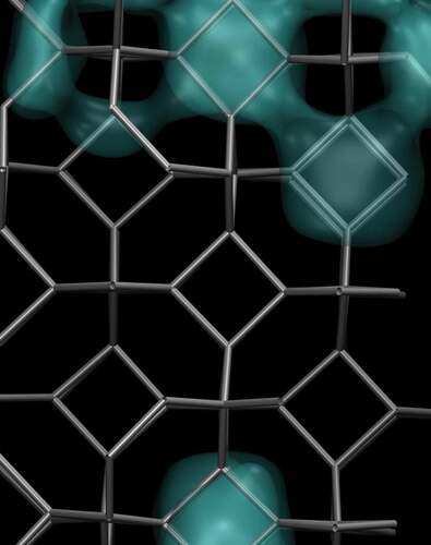
Figure 1. Definition of hydrophilic (left) and hydrophobic (right) solids depending on the contact angle ${\theta }_Y$: if ${\theta }_Y<{90}^{\circ }$, the solid is said hydrophobic, if ${\theta }_Y>{90}^{\circ }$, it is said hydrophilic.

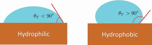
Figure 2. A) Liquid intruding a pore. Bulk and interface terms of Eq. 1 are shown graphically, together with the geometrical meaning of the contact Young angle ${\theta }_Y$. b) Graphical representation of the conditional (constant $V_B$) minimization of the grand potential vs ${\mathrm{\Sigma }}_{LB}$, thus obtaining the optimal liquid/bubble interface ${\mathrm{\Sigma }}_{LB}^{\ast }$. c) Sketch of the free energy/grand potential profile along intrusion. The system is initially extruded and $V_B$ is large; to intrude, the pore the liquid must cross a grand potential barrier much higher than the thermal energy, $k_{B}T$, which results in a large number of unsuccessful attempts (represented by the red arrow).

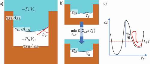
Figure 3. A) Liquid extrusion path according to cCNT. Dashed lines represent the LB interface at different stages along extrusion from a 2D square pore. b) Dependence of the intrusion (black) and extrusion (red) barrier as a function of the pressure. Here, for the sake of generality, both the pressure and barrier are dimensionless; $\mathrm{\Delta }\tilde{p}=\left(P_L-P_B\right)/\mathrm{\Delta }{p}_{max}$, with $\mathrm{\Delta }{p}_{max}=-2{\gamma }_{LB}cos{\vartheta }_Y/l$, where $l$ is the characteristic length of the texture (see panel a); $\mathrm{\Delta }{\omega }^{†}=\mathrm{\Delta }{\mathrm{\Omega }}^{†}/\left(V\mathrm{\Delta }{p}_{max}\right)$, where $\mathrm{\Delta }{\mathrm{\Omega }}^{†}$ is the transition barrier, from either Wenzel to Cassie-Baxter (W → CB) or vice versa (CB → W), and $V$ is the volume of the texture. In particular, in this panel, we show the intrusion/extrusion barrier as a function of the pressure for a system with ${\vartheta }_Y={110}^{\circ }$, a typical value of the so-called chemical hydrophobicity for materials of technological interest in the field of superhydrophobicity. c) extrusion time ${\tau }_{ext}$ as a function of the liquid pressure $P_L$ for a cubic pore of 10 nm characteristic length and ${\vartheta }_Y={126}^{\circ }$. The horizontal line corresponds to ${\tau }_{ext}=$ 1 s. d) Configurations along the liquid extrusion from the cavity of panel a) as obtained from the continuum string method. The blue region represents the liquid domain, which changes along the process. Adapted from Refs. [21] and [38].

Figure 4. Free energy, g(v), vs volume, V, of a vapor bubble in a bulk liquid as obtained by simulations (colored curves) and CNT including size dependence of the surface tension (dashed curves) at various values of the liquid pressure, reported aside the curves (Adapted from [53]).

Figure 5. Comparison between the free energy profile of a single variable, number of water molecules in a square 2D cavity (Figures 2, 3), or the corresponding liquid volume, for atomistic (RMD) and continuum (CREaM) models, vs the density profile $\rho \left(\mathrm{x}\right)$ (atomistic string), an atomistic proxy of the liquid/bubble interface ${\mathrm{\Sigma }}_{\mathrm{L}\mathrm{B}}$ (interface string). $\mathrm{\Delta }\omega =\mathrm{\Delta }\mathrm{\Omega }/\left(\mathrm{V}\mathrm{\Delta }{\mathrm{p}}_{\mathrm{m}\mathrm{a}\mathrm{x}}\right)$, with $\mathrm{\Delta }{\mathrm{p}}_{\mathrm{m}\mathrm{a}\mathrm{x}}=-2{\gamma }_{\mathrm{L}\mathrm{B}}cos{\vartheta }_{\mathrm{Y}}/\mathrm{l}$, where $\mathrm{l}$ is the characteristic length of the texture (see Figure 3). To make the comparison between the different calculations feasible, the free energy is reported as a function of the distance from the initial state, normalized for the total length of the path (normalized arc length). Here ‘distance’ is understood as the Euclidean distance in the space of the variables: N and $\rho \left(\mathrm{x}\right)$ for the atomistic calculations and ${\mathrm{V}}_{\mathrm{B}}$ and ${\mathrm{\Sigma }}_{\mathrm{L}\mathrm{B}}$ for the continuum ones. This distance has not an immediate and intuitive physical sense; rather, it is a measure of the separation between states of the system along the process, which is more conveniently represented in its normalized form, with values contained between 0 (initial state) and 1 (final state). Adapted from Refs. 28 and 45.

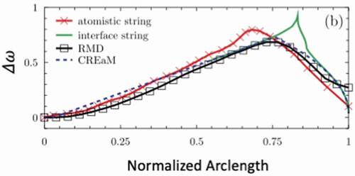
Figure 6. Free energy profile, in thermal units [k_BT], as a function of the number of water molecules between hydrophobic plates as obtained by INDUS. The free energy arbitrary constant is chosen such that the value at the filled (meta)stable state is zero. The relative stability of the filled and empty state and the barrier separating them depends on the distance between the plates. Adapted from Ref. [44].

Figure 7. Graphical illustration of the FFS method. Several trajectories are started from state A, at the center of the figure, and are continued only those reaching the first milestone, here illustrated as a prescribed distance from the center. From each note of the figure, representing the hit point of a trajectory with the next milestone, one starts several trajectories evolving according to a stochastic dynamics, which then can follow different paths. This operation is repeated until enough trajectories reach the final basin. The statistical analysis of these trajectories allows one to determine the process rate (see main text). Moreover, joining the piecewise trajectories allows one to investigate the mechanism of the process, to identify multiple ”reactive” channels, if present. Adapted from Ref. 44.

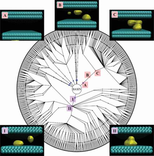
Figure 8. Intrusion/extrusion mechanism: comparison between the quasi-static and genuine dynamic paths as obtained from RMD and FFS, respectively. a,b) Intrusion/extrusion free energy profiles $\mathrm{\Delta }\mathrm{\Omega }$ as a function of the number of fluid particles within the 2D pore, N, c) at a set of pressures spanning the range in which the intruded and extruded states are the stable ones, and the process to go from the less to the more stable state is either characterized by a sizable barrier or its barrierless. Pressures are reported in Lennard-Jones reduced units of measure, $\epsilon /{\sigma }^3,$ where $\epsilon$ and $\sigma$ are the characteristic energy and length, respectively, the Lennard-Jones particles of the fluid. d) The mechanism is investigated considering the degree of symmetry of the liquid along intrusion, measured by the difference $N_1-N_2$ of fluid particles in the left and right halves of the pore. Panel d) shows that regardless of the pressure, if the process is studied in quasi-equilibrium conditions (RMD, INDUS and other methods), i.e. giving the system enough time to reach equilibrium at the present level of filling $N$, starting from ~60% of filling, the symmetry is broken, with more liquids in the left ($N_1-N_2>0)$ or right ($N_1-N_2<0$) half of the pore. This mechanism is followed regardless of the pressure, and intrusion and extrusion take place following the same path along opposite directions. (f-m) A similar analysis is shown for FFS simulations, which allow to take into account genuine dynamical effects (FFS). In this case, where we report the color map of the (logarithm) of the probability density to find the liquid in a configuration consistent with prescribed values of $N_1-N_2$ for a given total number of liquid particles in the cavity, $N$, along intrusion (f-h) and extrusion (i-m) trajectories at various pressures. The color code of the map is reported at the bottom of the figure. One notices that in this case i) intrusion and extrusion follow significantly different paths and ii) within each process, either intrusion or extrusion, the path depends on the pressure. These results stress the relevance of dynamical effects in intrusion/extrusion and the need to go beyond the quasi-static picture. Adapted from Ref. [90].

Figure 9. Color map of the density field of a liquid in contact with an hydrophobic surface with a 2D squared pore. The two panels show the two (meta)stable states of the liquid. The alternation of darker and lighter colors corresponds to local maxima and minima of the density field, the typical oscillation of the liquid density at hydrophobic walls.

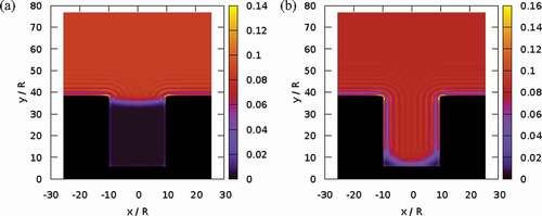
Figure 10. Left: Relevant states of the hydrophobic nanopore with diameter 14 Å (gray) immersed in water (blue) containing one argon atom (red). Right: free-energy profiles along two different paths connecting state A to state D. As customary in free energy calculations, the free energy is reported as the normalized arc length (see Figure 5), with values contained between 0 (initial state) and 1 (final state). The path A-C-D is the most likely drying path, characterized by two negligible free energy barriers. The right panel is reprinted with permission from Ref. 12.

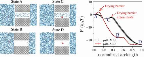
Figure 11. Scheme of intrusion–extrusion cycle. a) Negligible hysteresis loop (molecular spring), b) pronounced hysteresis (shock-absorber), c) irreversible intrusion: no extrusion at the lower end of operative pressures (bumper).

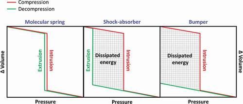
Figure 12. Sketch of an intrusion–extrusion porosimeter. A sample of lyophobic porous solid powder is placed in a liquid (in blue) and the pumps control the pressure of a pressure-transmitting fluid (in yellow). A manometer records the pressure P during the experiment, and a transducer records changes in volume of the system. The total change in the volume is then corrected for the compressibility of the non-wetting liquid and pressure transmitting fluid, in order to obtain the volume of non-wetting liquid intruded into the porous solid [117].

Figure 13. Scheme of PVT-calorimeter for recording heat of intrusion–extrusion: a differential scheme of the calorimeter implies two cells (measuring cell and reference cell), both of which have hermetic cone plugs and are directly connected to a high-pressure hydraulic line containing pressure-transmitting fluid. Both cells are identical and are filled with the same liquid. The porous material is inserted only into the measuring cell. To maintain the sample in place, a non-hermetic ampule is used. Flexible bellows are soldered to the lower ends of the cells. These bellows serve two purposes: i) separate the liquids from the pressure-transmitting fluid and ii) record volume variations of the sample via direct connection of the bellow to a LVDT system. The calorimeter is slide-down onto the cells, ensuring tight contact between the colorimetric detector and the cells. Calorimetric block is surrounded by a heating-cooling shield and passive thermal insulation. The heating of the cells is done via the heater, while cooling via circulation of the cooling fluid. Dry air is blown through the calorimeter during cooling to avoid condensation [119].

Figure 14. Different configurations of a high-pressure cell for recording electrification effects during intrusion–extrusion: a) hermetic flexible Teflon capsule containing two electrodes filled with a porous material and a (non-wetting) liquid. Porous material is maintained between the electrodes via Teflon tape. Rigid Teflon spacers are introduced between electrodes to ensure constant distance between them. b) Flexible Teflon tube is filled with the porous material and the (non-wetting) liquid. The two electrodes also serve as plugs of both ends of the tube. In both configurations, a and b, the capsule/tube is immersed in a pressure transmitting fluid. Using high-pressure through, wires connect electrodes to the recording equipment [6,126].

Figure 15. HLS car shock absorbers: a) prototypes of shock absorbers together with the PV intrusion/extrusion isotherm of the material used to dissipate mechanical energy [133]. The prototype in lab (b) [133] and field testing (c, d) [147] with and without Caron hydropneumatic suspensions (CHS)). In panel e), it is shown a comparison between the structural characteristics of conventional oil-based and HLS-based shock-absorber [148].

Figure 16. {Cu₂(tebpz) + water} molecular spring: a) PV-isotherms and b) VT-isobars intrusion–extrusion curves. The curves were shifted along the relative ΔV axis for clarity [129].

Figure 17. ZIF-8 + water system: (a) experimental evolution of lattice parameter a with pressure (the error bars are plotted on a 1σ confidence level). (b) PV-isotherm and contact angle; (c) topological model of cavity of ZIF-8; (d − f) schemes of framework response to compression before and during water intrusion, respectively. Here, the blue color represents water, while the black color is used to indicate the dimensions of the framework. (g) Theoretical evolution of lattice parameter a with pressure and (h) stroboscopic trajectory of two connected ZnIm4 tetrahedra, i.e. two tetrahedra sharing an Im ligand. One observes a counter-rotation of the two tetrahedra that makes the Zn−Im−Zn triad more colinear, which increases the Zn−Zn distance, hence the lattice size. Note, due to cubic symmetry of ZIF-8, all the lattice parameters are equal and evolve with pressure in a similar way [130].

Figure 18. Heating−cooling cycles of (a) {WC8 silica + water} (P₀ = 0.1 MPa) and (b) {ZIF-8 + water} (P₀ = 15 MPa) systems [136].

Figure 19. Calculated isobaric coefficient of thermal expansion of HLS [135].

Figure 20. Scheme of an RPLC chromatography. A liquid solution of the species to be analyzed is inserted, together with the eluent, in the RPLC column, which contains the stationary phase responsible for the differential retention of the various analytes. The typical output of an RPLC chromatography is a chromatogram showing the traces, peaks, obtained by the detector (e.g. a mass spectrometer) for various analytes. The area underneath these peaks is proportional to the concentration of the corresponding analyte in the original solution. The analyte is characterized by a specific retention time, the time from the beginning of the measurement at which the peak appears. In ideal conditions, RPLC should produce well-separated peaks in the chromatogram, resulting from a good separation of the various analytes.

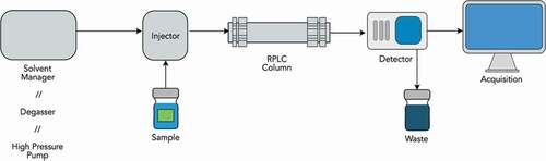
Figure 21. PV-isotherms (295 K) of water with (a) WC8, (b) ZIF-8, and (c) Cu2(tebpz) using different pressurization rates. d) Rate dependence of the water intrusion hysteresis as a function of porous material flexibility. Adapted from Ref. [126].

Figure 22. Thermal energy storage using melting–intrusion–extrusion–solidification cycle [124]. Initially, the PCM is solid and the porous material is extruded. Heat from the environment raises the temperature of the storage device above the melting temperature of the PCM, which melts. Any further increase of the temperature raises the pressure of the system, and when this reaches $P_{intrusion}$, the porous material gets intruded by the molten non-wetting PCM. This last step increases the energy that can be stored in the system. The heat stored along this ‘charging’ process is released to the environment along the reverse, ‘discharging’ path.

Cahn JW. Critical point wetting. J Chem Phys. 2008;66:3667.

 Google Scholar

Altabet YE, Haji-Akbari A, Debenedetti PG. Effect of material flexibility on the thermodynamics and kinetics of hydrophobically induced evaporation of water. Proc Natl Acad Sci. 2017;114:E2548–E2555.

 PubMed Web of Science ®Google Scholar

Menzl G, Gonzalez MA, Geiger P, et al. Molecular mechanism for cavitation in water under tension. Proc Natl Acad Sci. 2016;113:13582–13587.

 PubMed Web of Science ®Google Scholar

Giacomello A, Chinappi M, Meloni S, et al. Metastable wetting on superhydrophobic surfaces: continuum and atomistic views of the Cassie-Baxter–Wenzel transition. Phys Rev Lett. 2012;109:226102.

 PubMed Web of Science ®Google Scholar

Giacomello A, Meloni S, Müller M, et al. Mechanism of the Cassie-Wenzel transition via the atomistic and continuum string methods. J Chem Phys. 2015;142:104701.

 PubMed Web of Science ®Google Scholar

Remsing RC, Xi E, Vembanur S, et al. Pathways to dewetting in hydrophobic confinement. Proc Natl Acad Sci. 2015;112:8181–8186.

 PubMed Web of Science ®Google Scholar

Marchio S, Meloni S, Giacomello A, et al. Wetting and recovery of nano-patterned surfaces beyond the classical picture. Nanoscale. 2019;11:21458–21470.

 PubMed Web of Science ®Google Scholar

Giacomello A, Roth R. Bubble formation in nanopores: a matter of hydrophobicity, geometry, and size. Adv Phys X. 2020;5:1817780.

 Web of Science ®Google Scholar

Fraux G, Coudert F-X, Boutin A, et al. forced intrusion of water and aqueous solutions in microporous materials: from fundamental thermodynamics to energy storage devices. Chem Soc Rev. 2017;46:7421–7437.

 PubMed Web of Science ®Google Scholar

Grosu Y, Renaudin G, Eroshenko V, et al. Synergetic effect of temperature and pressure on energetic and structural characteristics of {zif-8 + water} molecular spring. Nanoscale. 2015;7:8803–8810.

 PubMed Web of Science ®Google Scholar

Grosu Y, Mierzwa M, Eroshenko VA, et al. Mechanical, thermal, and electrical energy storage in a single working body: electrification and thermal effects upon pressure-induced water intrusion-extrusion in nanoporous solids. ACS Appl Mater Interfaces. 2017;9:7044–7049.

 PubMed Web of Science ®Google Scholar

Lowe A, Tsyrin N, Chorażewski M, et al. Effect of flexibility and nanotriboelectrification on the dynamic reversibility of water intrusion into nanopores: pressure-transmitting fluid with frequency-dependent dissipation capability. ACS Appl Mater Interfaces. 2019;11:40842–40849.

 PubMed Web of Science ®Google Scholar

Eroshenko VA, Piatiletov I, Coiffard L, et al. A new paradigm of mechanical energy dissipation. part 2: experimental investigation and effectiveness of a novel car damper. Proc Inst Mech Eng Part D J Automob Eng. 2007;221:301–312.

 Web of Science ®Google Scholar

Suciu CV. Ride-comfort of an automobile equipped with colloidal dampers at its frontal suspensions. In Proceedings of ISMA 2010 - International Conference on Noise and Vibration Engineering, including USD 2010, Leuven (BE); 2010; p 4233.

 Google Scholar

Suciu CV, Buma S On the Structural Simplification, Compact and Light Design of a Vehicle Suspension, Achieved by Using a Colloidal Cylinder with a Dual Function of Absorber and Compression-Spring. In FISITA 2012 World Automotive Congress, Beijing; 2013.

 Google Scholar

Chorążewski M, Zajdel P, Feng T, et al. Compact thermal actuation by water and flexible hydrophobic nanopore. ACS Nano. 2021;15:9048–9056.

 PubMed Web of Science ®Google Scholar

Tortora M, Zajdel Pawełand Lowe AR, Chorażewski M, et al. others. giant negative compressibility by liquid intrusion into superhydrophobic flexible nanoporous frameworks. Nano Lett. 2021;21:2848.

 PubMed Web of Science ®Google Scholar

Eroshenko V, Grosu Y, Tsyrin N, et al. Exceptionally large and controlled effect of negative thermal expansion in porous heterogeneous lyophobic systems. J Phys Chem C. 2015;119:19.

 Web of Science ®Google Scholar

Grosu Y, Faik A, Nedelec J-M, et al. Reversible wetting in nanopores for thermal expansivity control: from extreme dilatation to unprecedented negative thermal expansion. J Phys Chem C. 2017;121:21.

 Web of Science ®Google Scholar

Lowe AR, Wong WSY, Tsyrin N, et al. The effect of surface entropy on the heat of non-wetting liquid intrusion into nanopores. Langmuir. 2021;37:4827–4835.

 PubMed Web of Science ®Google Scholar