Berry phase in quantum oscillations of topological materials

Figures & data

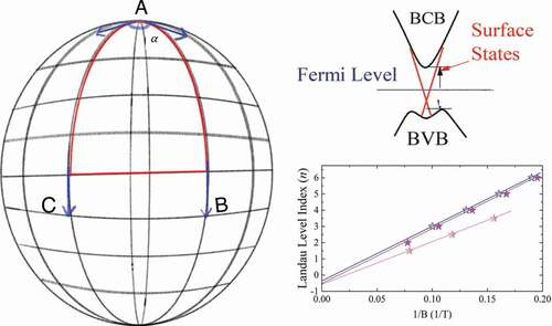
Figure 1. Illustration of the geometrical phase generated along a closed path on a surface. (a) The geometric phase of a vector moving on a sphere. Initially at the north pole, the vector is parallel-transported along the longitude AB to the equator BC, and then to the longitude CA. Even though the vector has not been rotated at any point along its route, it has been rotated at an angle α. The angle α is the integral of the Gaussian curvature К over the area enclosed by the route. (b) The adiabatic evolution of a quantum state $\left|n\left(R\right)\right.⟩$ along a smooth circuit in the parameter space. The quantum parallel transport of a state means that $n|\frac{d}{dt}|n=0$, namely, the change of a state cannot be along its own direction. After returning to the starting point, the state is rotated and acquires the Berry phase γ_n(C), which is the integral of the Berry curvature Ω_n over the area S.

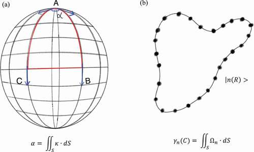
Figure 2. The reshaped Fermi surface from a sphere to Landau tubes.

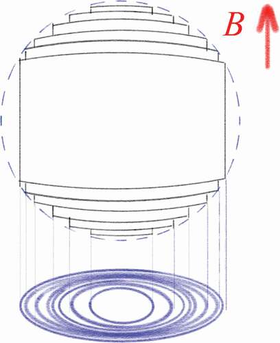
Figure 3. Band structures and the related Fermi surfaces of metals: normal metal, Dirac semimetal, Weyl semimetal, and topological nodal-line semimetal [34].

Figure 4. Quantized magnetoresistance and Hall resistance of a graphene device. a, Hall resistance and magnetoresistance measured at 30 mK and gate voltage, V_g = 15 V. The vertical arrows and the numbers on them indicate the values of magnetic field and the corresponding filling factors of quantum Hall states. The horizontal lines correspond to h/e² values. The inset shows the QHE for a hole gas at V_g = −4 V, measured at 1.6 K. The quantized plateau for the filling factor ν = 2 is well-defined, and the second and the third plateaus with ν = 6 and 10, respectively, are also resolved. b, The Hall resistance (black) and magnetoresistance (Orange) as functions of gate voltage at fixed magnetic field B = 9 T, measured at 1.6 K. The same conventions as in a are used here. The upper inset shows a detailed view of high filling factor plateaus measured at 30 mK. c, A schematic diagram of the Landau level (LL) density of states (DOS) and corresponding quantum Hall conductance (σ_xy) as functions of energy. Note that in the quantum Hall states, σ_xy = -R_xy⁻¹. The LL index n is shown next to the DOS peak. In the experiment, the Fermi energy E_F can be adjusted by the gate voltage, and R_xy⁻¹ changes by the amount of g_se²/h as E_F crosses a LL, where g_s accounts for the spin and valley degeneracies [51].

Figure 5. Local Berry phase measurement technique by scanning tunneling microscope (STM). (a) The STM setup, in which the DOS of 2D systems can be directly probed over a wide energy range. (b) Landau level spectra of monolayer graphene in various magnetic fields (4–12 T). The monolayer graphene was decoupled from its multilayer graphene substrate. The data are offset on the Y axis for clarity, and the top labels are the Landau level indices. (c) Landau level energies extracted from panel (b) versus sgn(n)(|n|B)^1/2. (c) Energy-fixed DOS as functions of magnetic field for different tunneling biases V_B. (d) Fan plot showing linear dependences of the Landau level indices, taken from the DOS oscillations in monolayer graphene versus 1/B for different tunneling biases. Points n, (n  1/2) are associated with the n^th minima (maxima) of the DOS oscillations. The solid lines are the linear fitting results of the slope BE. Their n-axis intercepts (panel (e)) directly reflect a Berry phase of π in the monolayer graphene. Panel (e) also plots the intercepts in pristine monolayer graphene versus the back gate voltage V_g (top x-axis) [56].

Figure 6. (A) Derivative dr_yx/dH versus 1/H in sample Q3 measured at temperatures T between 0.3 and 20 K. (B) The conductance obtained after subtracting a smooth background based on curves measured above 20 K (ΔG) for sample Q2 at selected T over the same interval. (C) LL index plot of 1/H versus n for samples Q1, Q2, and Q3. The results are consistent with 0 < γ < 1/2. (D) T dependence of the normalized conductivity amplitude at 0.3 K in samples Q2 (with H = 12 T) and Q3 (7.8 T). Dingle plots used to determine quantum relaxation time for (E) sample Q2 and (F) sample Q3 [69].

Figure 7. (a) The longitudinal resistivity of a Cd₃As₂ single crystal in zero magnetic field, with current in the (112) plane. A typical X-ray rocking curve of the (224) Bragg peak is shown in the inset. (b) The Hall resistance R_xy at 200, 100, 50, and 1.5 K. There are clear oscillations of R_xy at 1.5 K, as seen in the inset. (c) The Shubinikov – de Haas oscillations of longitudinal magnetoresistance (MR) at various temperatures, with the field perpendicular to the (112) planes. At 280 K, the MR is roughly linear without saturation, as high as 200% at B = 14.5 T. At 1.5 K, the oscillations appear at a field as low as 2 T, reflecting the high mobility of charge carriers in Cd₃As₂. (d) The high-field oscillatory components ΔR_xx and ΔR_xy at 1.5 K. The ΔR_xy oscillations are phase shifted by approximately 90° with respect to the ΔR_xx oscillations for the low Landau levels. No Landau level splitting is observed in the field range. (e) Landau index n plotted against 1/B. The closed circles denote the integer index (ΔR_xx valley), and the open circles indicate the half integer index (ΔR_xx peak). The index plot can be linearly fitted, giving an intercept of 0.58. The measurements of another single crystal labeled as sample B give a similar intercept of 0.56. From the inset, both intercepts of ΔR_xx lie between 1/2 and 5/8, which is strong evidence for a nontrivial π Berry’s phase of 3D Dirac fermions in Cd₃As₂ [86].

Figure 8. Temperature dependence of the Hall resistivity and resistivity for TaAs. (a) The Hall resistivity measured at various temperatures from 2 to 300 K. The lower-left and the upper-right insets show the Hall resistivity at 2 and 300 K, respectively. The obvious SdH oscillations demonstrate the high quality of the sample. (b) The Hall resistivity at T = 90, 100, 120, and 150 K. (c) Temperature dependence of the carrier mobility μ_e and μ_h of electrons and holes deduced by the two-carrier model. Main panel: Fitting with σ_xy; inset: fitting with σ_xx. (d) Magnetic field dependence of the resistivity with θ = 0° at representative temperatures. (e) Main panel: Oscillatory components of ρ_xx at 1.8 K, obtained by subtracting the ρ_xx at 20 K. The open circles are the experimental data, and the red line is the best fit based on two oscillatory frequency components. Upper inset: The two frequency components extracted from the raw oscillation patterns in the main panel. Lower inset: Landau-level index plots of 1/B versus n for different oscillation frequencies. (f) The temperature dependence of the resistivity in a magnetic field perpendicular to the electric current. The red arrow indicates that the resistivity peak moves to high temperatures under higher magnetic fields. The inset gives the measurement configuration and zooms in on the case of 0 T [89].

Figure 9. Quantum oscillation study of Co₃Sn₂S₂. (a, e) Magnetoresistance as a function of the magnetic field μ₀H at different temperatures for H ∥ z-axis and H ∥ y-axis, respectively. (b, f) The oscillatory part of the resistivity Δρ for H ∥ z-axis and H ∥ y-axis, respectively. (c, g) Fast Fourier transform spectra at various temperatures. The inset shows the multi-peak fitting used to distinguish between superposed frequencies. (d, h) The LK fitting with the effective masses [109].

Figure 10. (A and B) SdH oscillations obtained by subtracting the smooth background from the MR measurements, plotted against inverse magnetic field (1/B) at different temperatures for the two deconvoluted components. The A and B insets show the corresponding FFT results. (C) The angular dependence of oscillation frequencies. For clarity, FFT results for different angles are shifted vertically. A schematic diagram of the experimental setup is shown in the inset. (D) Temperature dependence of the relative amplitude of SdH oscillations for both the Fermi pockets. (E) Landau-level index plot for the 238 T frequency oscillation, with the arrow showing the value of the y-axis intercept. The inset shows the x-axis intercept for the extrapolated linear fitting [115].

Figure 11. Non-trivial Berry phase of topological fermions in Sr_1-yMn_1-zSb₂. a, The in-plane longitudinal and transverse (Hall) resistivities as functions of magnetic field measured at 2 K on a similar sample, A4; both ρ_xx and ρ_xy show strong SdH oscillations. b, The in-plane conductivity converted from the ρ_xx and ρ_xy data. c, The in-plane oscillatory conductivity Δσ_xx versus 1/B at 2 K. d, The Landau Level (LL) index fan diagram derived from the oscillatory conductivity at 2 K of sample A4. The integer LL indices (n) are assigned to the minima of Δσ_xx. The intercept n₀ on the n axis obtained from the extrapolation of the best linear fit in the fan diagram is at n = 0.55 ± 0.02, suggesting that the π Berry phase has accumulated in the cyclotron orbits. e, FFT spectrum of the in-plane conductivity σ_xx at 2 K for sample A4. f, Fit of the dHvA oscillation pattern at 2 K to the LK formula (see the Methods) for sample C1, from which non-trivial Berry phases were also obtained [116].

Weng H, Dai X, Fang Z. Topological semimetals predicted from first-principles calculations. J Phys. 2016;28:303001.

 Google Scholar

Zhang YB, Tan YW, Stormer HL, et al. Experimental observation of the quantum Hall effect and Berry’s phase in graphene. Nature. 2005;438:201–204.

 PubMed Web of Science ®Google Scholar

Ren Y-N, Zhang M-H, Yan C, et al. Local measurements of tunneling magneto-conductance oscillations in monolayer, Bernal-stacked bilayer, and ABC-stacked trilayer graphene. Sci China Phys Mech Astron. 2021;64:1–6.

 Web of Science ®Google Scholar

Qu D-X, Hor YS, Xiong J, et al. Quantum oscillations and Hall anomaly of surface states in the topological insulator Bi2Te3. Science. 2010;329:821–824.

 PubMed Web of Science ®Google Scholar

He L, Hong X, Dong J, et al. Quantum transport evidence for the three-dimensional Dirac semimetal phase in Cd3As2. Phys Rev Lett. 2014;113:246402.

 PubMed Web of Science ®Google Scholar

Huang XC, Zhao LX, Long YJ, et al. Observation of the Chiral-Anomaly-Induced Negative Magnetoresistance in 3D Weyl Semimetal TaAs. Phys Rev X. 2015;5:031023.

 Web of Science ®Google Scholar

Ding L, Koo J, Yi C, et al. Quantum oscillations, magnetic breakdown and thermal Hall effect in Co3Sn2S2. J Phys D Appl Phys. 2021;54:454003.

 Web of Science ®Google Scholar

Singha R, Pariari AK, Satpati B, et al., Large nonsaturating magnetoresistance and signature of nondegenerate Dirac nodes in ZrSiS, Proceedings of the National Academy of Sciences U.S.A., 114 (2017) 2468–2473.

 Google Scholar

Liu J, Hu J, Zhang Q, et al. A magnetic topological semimetal Sr1−yMn1−zSb2 (y, z < 0.1). Nat Mater. 2017;16:905–910.

 PubMed Web of Science ®Google Scholar