Recent advances on time-stretch dispersive Fourier transform and its applications

Figures & data

Figure 1. Schematic illustration of the space-time duality in optics: The equivalence between the diffraction (spatial domain) and dispersion (temporal domain) phenomena summarizes the physical concepts underlying the frequency-to-time mapping approach used in the ‘Dispersive Fourier transform’ technique as well as its implementation for the realization of so-called ‘Time-lens’ measurements. (a) Diffraction of light through a circular aperture. (b) Convergent lens and the construction of an enlarged image. (c) Principle of the dispersive Fourier transform technique, allowing to readily map the broadband spectrum of a pulsed light source in the temporal domain. (d) Principle of the time lens, allowing for the magnification of the temporal optical waveform by the concatenation of two dispersive elements separated by an element used to apply a quadratic temporal phase on the optical waveform (i.e. a lens in the temporal domain).

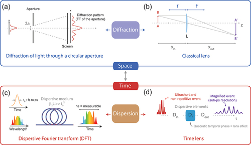
Figure 2. Principle of DFT measurements. (a) A broadband optical signal is temporally stretched after linear propagation in a highly dispersive fiber. The various spectral components of the optical signal are mapped in the temporal domain so that the optical spectrum can be directly retrieved from the pulse temporal intensity waveform. (b) For the retrieval and analysis of non-repetitive events, real-time spectra from different pulses can be directly acquired from ultrafast optoelectronic measurements (e.g. using a > GHz photodiode + oscilloscope detection system) with the ability to readily analyze shot-to-shot fluctuations from successive traces. In this case, the equivalent DFT spectral resolution is related to the bandwidth of the detection system as well as the magnitude of DFT time-stretch. The achievable resolution is thus a tradeoff between the digitizer sampling rate, the spectral bandwidth of the broadband optical signal and the pulse train repetition rate (to avoid any temporal overlap between adjacent time-stretched spectra).

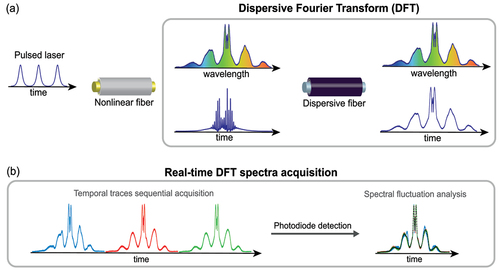
Figure 3. Typical DFT results for the real-time characterization and statistical analysis of spectral fluctuations in nonlinear fiber optics. The DFT technique, via the setup shown in (a), can be used to study a variety of dynamics highly sensitive to noise fluctuations, from a fully developed broadband incoherent supercontinuum (top) to, e.g., the onset phase of nonlinear propagation where spontaneous modulation instability takes place (bottom): (b) DFT experimental characterization of an extended incoherent supercontinuum, exhibiting important shot-to-shot spectral fluctuations. (c,d) The spectral intensity histograms reconstructed at different wavelengths exhibit very different distributions and illustrate how particular spectral regions are prone to the appearance of statistically rare ‘extreme’ events. (e) Spectral fluctuations of MI sidebands sequentially recorded by DFT. The statistical analysis of these fluctuations can be leveraged to reconstruct a map of spectral correlation (f) that can be directly compared to the same Pearson correlation maps obtained from stochastic Monte-Carlo simulations (g). Adapted from Ref. [24].

Figure 4. Example of DFT implementation for the experimental analysis of octave-spanning supercontinuum: (a) Experimental setup. (b) Single shot spectra obtained experimentally by DFT measurements. (c) Superimposed single shot (grey dashes) and mean (black line) DFT spectra obtained from real-time DFT measurement and compared to optical spectral analyzer ‘averaged’ measurement (red dashes). (d) Octave spanning spectral correlation map (via Pearson coefficient) reconstructed form experimental DFT shot-to-shot spectral fluctuation analysis. Adapted from Ref. [62].

Figure 5. Sea of random picosecond pulses, as typically generated via modulation instability during nonlinear fiber propagation (results obtained from numerical GNLSE simulations [68]). Resolving such non-repetitive pulses would theoretically require a direct detection with a bandwidth close to THz values, a figure out of the range of current electronic detectors.

Figure 6. Schematic of an experimental setup used for the characterization of random picosecond pulses (breathers) as generated after nonlinear fiber propagation of a noisy continuous wave input (see Figure 5). The time lens uses two dispersive propagation steps (D₁ and D₂), one on each side of an element that applies a quadratic temporal phase. In this experiment, the quadratic phase was applied from four wave mixing (FWM) with a linearly chirped pump pulse co-propagating in a silicon waveguide. The 90 ps chirped pump pulses are generated from a femtosecond pulse subsequently stretched through propagation in a fiber of dispersion D_p. The wavelength-converted idler after FWM (with applied quadratic phase) is filtered before further propagation in segment D₂. The overall temporal magnification is 76.4 such that the temporally stretched replica can be resolved using a 30 GHz bandwidth detection system. Adapted from Ref. [73].

Figure 7. Examples of fiber laser evolution dynamics characterized via DFT analysis over hundreds of cavity roundtrips. (a) Experimental setup for the study of a fiber laser exhibiting soliton-similariton dynamics via DFT. (b) Single pulse mode-locking obtained after a transition from a noisy operation and an explosion regime (white dashed box), with an abrupt spectral broadening clearly captured by DFT measurements. (c) DFT measurements can be used to study the dynamical evolution of a soliton molecular state. The spectra evolution can be used to retrieve autocorrelations of the field, stemming from a ‘molecule state’ with a periodically oscillating phase. Panels (a-c) are adapted from [91]. (d) Experimental observation of the Sagnac effect in a bidirectional fiber laser, illustrated by a change in the tilted modulation pattern within the DFT spectra. Adapted from [103].

Figure 8. Capturing FOPO dynamics using DFT. (a) Experimental setup of the fiber optical parametric oscillator under study. C: couplers, CIRC: optical circulator, DSF, dispersion shifted fiber, EDFA: erbium-doped fiber amplifier. (b) Typical MI-LSQ map constructed from ~2000 consecutive shot-to-shot spectra. (c) Specific dynamical behaviour obtained when increasing the pump intensity fluctuations. Reproduced from Ref. [107].

Figure 9. DFT characterization of high repetition-rate frequency combs. (a) Microcomb generation: A Laser Cavity-Solitons train is emitted from a microresonator nested in a fiber cavity. Modulated Dispersive Fourier Transform: the repetition rate of the pulse train is reduced using an electro-optic modulator connected to a pulse generator (1,2). DFT is then achieved through a DCF (3) and data is processed using a fast oscilloscope. (b) Typical DFT-plot of a Turing pattern, startup and stable regime over 2000 roundtrips. Optical spectrum analyzer plot on the right for comparison [109].

Figure 10. Capturing ultrafast phenomena using DFT-based imaging. (a) Time-stretch imaging setup. (b) Snapshot of a typical laser-induced SW recorded using shadowgraphy. (c) Signal of a single SW: consecutive pulses are stacked horizontally (time axis), while positions (i.e. wavelengths) are displayed vertically. (d) Close-up on the shock wave and (e) corresponding velocities measurements. Reproduced from [113].

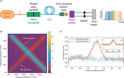
Figure 11. (a) Experimental setup to implement quantum DFT employed for spectral characterization of photon pairs created in pulsed-excited SPDC process in a PPLN waveguide. (b) Joint Spectral Intensity (JSI) determined by quantum DFT: CAR versus signal and idler frequency. (c) Coincidence detection as a function of the frequency difference $\mathrm{\Delta }\nu$ between the spectral components of the signal photon. The inset figure illustrates the dependency of $g^{\left(2\right)}\left(\mathrm{\Delta }\nu \right)$ on frequency difference, $\mathrm{\Delta }\nu$.

Wetzel B, Stefani A, Larger L, et al. Real-time full bandwidth measurement of spectral noise in supercontinuum generation. Sci Rep. 2012;2:882.

 PubMed Web of Science ®Google Scholar

Godin T, Wetzel B, Sylvestre T, et al. Real time noise and wavelength correlations in octave-spanning supercontinuum generation. Opt Express. 2013;21:18452.

 PubMed Web of Science ®Google Scholar

Dudley JM, Genty G, Coen S. Supercontinuum generation in photonic crystal fiber. Rev Mod Phys. 2006;78:1135.

 Web of Science ®Google Scholar

Närhi M, Wetzel B, Billet C, et al. Real-time measurements of spontaneous breathers and rogue wave events in optical fibre modulation instability. Nat Commun. 2016;7:13675.

 PubMed Web of Science ®Google Scholar

Lapre C, Billet C, Meng F, et al. Real-time characterization of spectral instabilities in a mode-locked fibre laser exhibiting soliton-similariton dynamics. Sci Rep. 2019;9. DOI:10.1038/s41598-019-50022-5

 PubMed Web of Science ®Google Scholar

Chernysheva M, Sugavanam S, Turitsyn S. Real-time observation of the optical Sagnac effect in ultrafast bidirectional fibre lasers. APL Photonics. 2020;5:016104.

 Web of Science ®Google Scholar

Touil M, Becheker R, Godin T, et al. Spectral Correlations in a Fiber-Optical Parametric Oscillator. Phys Rev A. 2021;103:043503.

 Web of Science ®Google Scholar

Hanzard PH, Rowley M, Cutrona A, et al., Real-time study of coexisting states in laser cavity solitons, in conference on lasers and electro-optics (2021), Paper FM4H.7 San Jose, California, United States (Optical Society of America), p. FM4H.7.

 Google Scholar

Hanzard P-H, Godin T, Idlahcen S, et al. Real-time tracking of single shockwaves via amplified time-stretch imaging. Appl Phys Lett. 2018;112:161106.

 Web of Science ®Google Scholar