Ultrafast dynamics of electrons and phonons: from the two-temperature model to the time-dependent Boltzmann equation

Figures & data

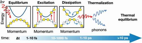
Figure 1. Schematic representation of two thermal reservoirs at temperatures $T_1$ and $T_2>T_1$ and energies $E_1=C_1{T}_1$ and $E_2=C_2{T}_2$ – where $C_1$ and $C_2$ denote the heat capacities – in absence of interactions (a), in presence of mutual interactions characterized by a coupling constant $g$ (c), and in presence of an external field (e). (b), (d), and (f): Time dependence of the temperature for the systems in (a), (c), and (e), respectively, as obtained from the solution of the TTM.

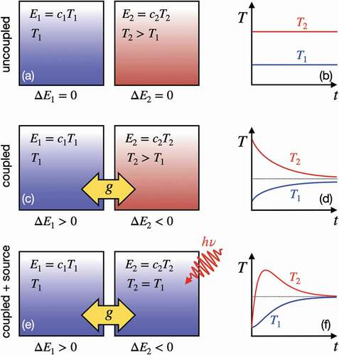
Figure 2. (a) Schematic illustration of the TTM and (b) NLM. At variance with the TTM, the NLM accounts for coupling with different subsets of phonon modes, as well as phonon-phonon interactions. (c) Time-dependence of the electronic (blue) and vibrational temperatures of the longitudinal (LA) and transverse acoustic phonons (TA₁ and TA₂) of aluminum. Reproduced from Ref [40].

Figure 3. Electron distribution function $f_{n\mathbf{k}}$ superimposed to the band structure of monolayer MoS₂. Energies are relative to the Fermi level. At equilibrium (left), bands are occupied according to the Fermi-Dirac statistics (Eq. (12)(12) $f_{n\mathbf{k}}^0(T)={\left[e^{({\epsilon }_{n\mathbf{k}}-{\epsilon }_{\mathrm{F}})/k_{\mathrm{B}}T}+1\right]}^{-1},$(12) ). Adapted from Ref [144].

Figure 4. Diagrammatic representation of (a) phonon-emission and (b) phonon-absorption processes. Wavy lines represent non-interacting phonon propagator, whereas straight lines denote non-interacting single-particle propagators. In both diagrams, time increases from left to right.

Figure 5. Schematic representation of the four phonon-assisted scattering processes included in the electron collision integral due to the electron-phonon interaction (Eq. (25)(25) $\begin{array}{rl}& {\mathrm{\Gamma }}_{n\mathbf{k}}^{\mathrm{e}\mathrm{p}}(t)=\frac{2\pi }{\mathrm{\hslash }{N}_p}\sum _{m\nu \mathbf{q}}|g_{mn}^{\nu }(\mathbf{k},\mathbf{q}){|}^2\\ & \times \{(1-f_{n\mathbf{k}})f_{m\mathbf{k}+\mathbf{q}}\delta ({\epsilon }_{n\mathbf{k}}-{\epsilon }_{m\mathbf{k}+\mathbf{q}}+\mathrm{\hslash }{\omega }_{\mathbf{q}\nu })(1+n_{\mathbf{q}\nu })\\ & +(1-f_{n\mathbf{k}})f_{m\mathbf{k}+\mathbf{q}}\delta ({\epsilon }_{n\mathbf{k}}-{\epsilon }_{m\mathbf{k}+\mathbf{q}}-\mathrm{\hslash }{\omega }_{\mathbf{q}\nu })n_{\mathbf{q}\nu }\\ & -f_{n\mathbf{k}}(1-f_{m\mathbf{k}+\mathbf{q}})\delta ({\epsilon }_{n\mathbf{k}}-{\epsilon }_{m\mathbf{k}+\mathbf{q}}-\mathrm{\hslash }{\omega }_{\mathbf{q}\nu })(1+n_{\mathbf{q}\nu })\\ & -f_{n\mathbf{k}}(1-f_{m\mathbf{k}+\mathbf{q}})\delta ({\epsilon }_{n\mathbf{k}}-{\epsilon }_{m\mathbf{k}+\mathbf{q}}+\mathrm{\hslash }{\omega }_{\mathbf{q}\nu })n_{\mathbf{q}\nu }\}.\end{array}$(25) ). Adapted from Ref [8].

Figure 6. (a) Schematic representation of the thermalization dynamics of electrons and holes following photo-excitation in the vicinity of the Dirac cone of graphene. Time and angle-resolved photoemission spectral function of doped graphene before photo-excitation (b), and at time delays $t=30$ fs (c), and $t=1$ ps (d). Momentum integrated spectral function (e) and, superimposed as a continuous line, the Fermi-Dirac function at the effective electronic temperature $T_e$. (f) Time-dependent effective electronic temperature derived by the fitting procedure illustrated in (e). Adapted from Ref [79].

Figure 7. (a) DFT Band structure of graphene in the vicinity of the Dirac cone along the M-K high-symmetry path in the Brillouin zone. (b) Left: Phonon dispersion of graphene obtained from DFPT. Right: Phonon density of states ($F$) and Eliashberg function (${\alpha }^{2}F$) of graphene. The peaks at 0.16 and 0.19 eV reflect the strong coupling to transverse optical (TO) and longitudinal optical (LO) phonons in the vicinity of the K and $\mathrm{\Gamma }$ points, respectively [green dots in panel (b)]. (c-d) Pump-probe photoemission measurements of the effective electronic temperature $T_{\mathrm{e}\mathrm{l}}$ of graphene (dots) for photo-excitation fluences $F=8\mathrm{J}/{\mathrm{m}}^2$ (c) and (d) $F=3.46\mathrm{J}/{\mathrm{m}}^2$ from Refs. [78,79]. Simulations based on the NLM (more precisely, three-temperature model) with first-principles parameters are reported as continuous lines. Panels (a-b) and (c-d) are adapted from Ref. [70] and Ref. [81], respectively.

Figure 8. (a) DFT Band structure of graphene in the vicinity of the Dirac cone. The dashed line denotes the Fermi energy ${\epsilon }_{\mathrm{F}}=-0.2$ eV, corresponding to a carrier concentration $8\times {10}^{12}$ cm ${ }^{-2}$. The inset illustrates the hexagonal Brillouin zone. First-principles calculations of the time- and angle-resolved spectral function obtained by considering electronic and vibrational occupations derived from the solution of the TTM before excitation (b), and at time delays $\mathrm{\Delta }t=0$ (c), $\mathrm{\Delta }t=0.5$ ps (d), and $\mathrm{\Delta }t=2.5$ ps (e). Reproduced from Ref [81].

Figure 9. Population of excited electrons and holes for an initial electronic excitation (a) superimposed to the band structure of graphene, and at subsequent time steps throughout the non-equilibrium dynamics as obtained from the solution of the time-dependent Boltzmann equation (b-c). The left panels denote the density of states of electrons and holes. (d-f) Time-dependent phonon distribution functions $n_{\mathbf{q}\nu }(t)$ superimposed to the phonon dispersion for several snapshot, with the point size being proportional to $n_{\mathbf{q}\nu }(t)$. (g) Energy resolved phonon population $n_{\mathbf{q}\nu }(t)$ as a function of time. Reproduced from Ref [143].

Figure 10. (a) Hexagonal Brillouin zone and high-symmetry points (dots) of monolayer MoS${ }_2$. The color coding reflects the effective vibrational temperature of the lattice for an initial ($t=0$) state of thermal equilibrium at $T=100$ K (see color bar). (b-e) Enhancement of the phonon temperature in the vicinity of the Γ and K high-symmetry points due to momentum-selective phonon emission throughout the relaxation of a photo-excited electronic distribution. Reproduced from Ref [223].

Waldecker L, Bertoni R, Ernstorfer R, et al. Electron-phonon coupling and energy flow in a simple metal beyond the two-temperature approximation. Phys Rev X. 2016 Apr;6:021003.

 Web of Science ®Google Scholar

Caruso F. Nonequilibrium lattice dynamics in monolayer mos2. J Phys Chem Lett. 2021;12:1734–1740. PMID: 33569950.

 PubMed Web of Science ®Google Scholar

Poncé S, Wenbin L, Reichardt S, et al. First-principles calculations of charge carrier mobility and conductivity in bulk semiconductors and two-dimensional materials. Rep Prog Phys. 2020 Feb;83:036501.

 PubMed Web of Science ®Google Scholar

Gierz I, Petersen JC, Mitrano M, et al. Snapshots of non-equilibrium dirac carrier distributions in graphene. Nat Mater. 2013 Dec;12:1119–1124.

 PubMed Web of Science ®Google Scholar

Christian Johannsen J, Ulstrup S, Cilento F, et al. Direct view of hot carrier dynamics in graphene. Phys Rev Lett. 2013 July;111:027403.

 PubMed Web of Science ®Google Scholar

Novko D. First-principles study of ultrafast dynamics of dirac plasmon in graphene. New J Phys. 2021 Apr;23:043023.

 Web of Science ®Google Scholar

Caruso F, Novko D, Draxl C. Photoemission signatures of nonequilibrium carrier dynamics from first principles. Phys Rev B. 2020 Jan;101:035128.

 Web of Science ®Google Scholar

Tong X, Bernardi M. Toward precise simulations of the coupled ultrafast dynamics of electrons and atomic vibrations in materials. Phys Rev Res. 2021 April;3:023072.

 Google Scholar

Caruso F. Nonequilibrium lattice dynamics in monolayer mos2. J Phys Chem Lett. 2021;12:1734–1740. 10.1021/acs.jpclett.0c03616.

 PubMed Web of Science ®Google Scholar