A review on non-Hermitian skin effect

Figures & data

Figure 1. (a) The HN model. (b) The energy band under PBC. (c-d) Mode profiles of all the eigenstates under OBCs. The total number of sites (i.e. the chain length) is taken as $N=30$.

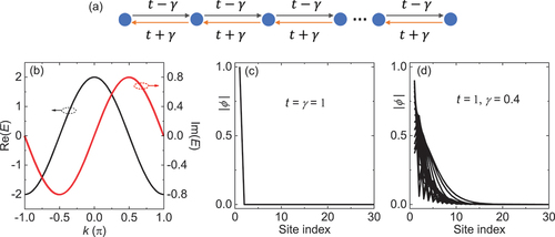
Figure 2. Sketches of (a) a regular and (b) a third-order EPs in gain/loss-induced two-level and three-level non-Hermitian systems. (c-d) Higher-order EPs emerging in the HN model with OBCs.

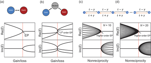
Figure 3. Energy windings under PBC for (a) the HN model with $t=1$, $\gamma =0.4$ and (b) its Hermitian counterpart. (c) The corresponding energy spectrum under OBC for the HN model in (a). (d-f) BZ and GBZ, periodic- and open-boundary spectra, together with the eigenmode distributions, for several non-Hermitian models yielding different GBZs. (d-f) are reproduced with permissions from Ref [44].

Figure 4. (a) The Hermitian SSH model, its energy spectra under (b-d) PBC and (e) OBC. (f-i) Mode profiles for the bulk and edge states. (j-r) The same as (a-i), only for the non-Hermitian SSH model. The figures are adapted with permissions from Ref [152].

Figure 5. Higher dimensional extensions of the HN model. The Orange shading schematically represents the distributions of the skin modes. Note that only the primary hopping is indicated for the sake of clarity.

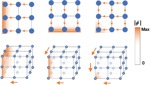
Figure 6. (a) The 2D tight-binding model, where NHSE is manifested as (b) corner skin modes for nonreciprocity in both directions and as (c) edge skin modes when nonreciprocity is canceled in the x-direction. (d-e) Hybrid skin-topological modes with nonreciprocity canceled in both directions. The figures are reproduced with permissions from Ref [96].

Figure 7. (a) Twisted windings in the HN model with long-range coupling and its bipolar skin effect. (b-d) Various windings by manipulating the long-range couplings. The figures are reproduced with permissions from Refs. [115,124].

Figure 8. (a) Experimental set-up of the optical fiber loops. (b) Time-modulation to realize nonreciprocal couplings. (c) A schematic light funnel proposed using the NHSE, whose experimental measurements are shown in (d-f) for different input of light. The figures are reproduced with permissions from Ref [128].

Figure 9. Experimental set-ups for NHSE demonstrations in various physical platforms, including (a) quantum-walks, (b) photonic synthetic dimensions, (c-f) 1D, 2D and 3D electric circuits, as well as (g) acoustic cavities equipped with electrical amplifiers. These figures are reproduced with permissions from Refs. [115,124,129,130,133,135].

Figure 10. A unit cell of the 2D reciprocal lattice. The green areas represent the lossy domains. (b) Nonreciprocal propagation for each clockwise or anticlockwise mode. (c) NHSE manifested as pseudospin-dependent corner skin modes. (d) The Hermitian case as the comparison. (a, c-d) are reproduced from Ref [121].

Zhang K, Yang Z, Fang C. Correspondence between winding numbers and skin modes in non-Hermitian systems. Phys Rev Lett. 2020;125:126402.

 PubMed Web of Science ®Google Scholar

Cheng J, Zhang X, Lu MH, et al. Competition between band topology and non-Hermiticity. Phys Rev B. 2022;105:094103.

 Web of Science ®Google Scholar

Lee CH, Li L, Gong J. Hybrid higher-order skin-topological modes in nonreciprocal systems. Phys Rev Lett. 2019;123:016805.

 PubMed Web of Science ®Google Scholar

Wang K, Dutt A, Yang KY, et al. Generating arbitrary topological windings of a non-Hermitian band. Science. 2021;371:1240–1245.

 PubMed Web of Science ®Google Scholar

Zhang L, Yang Y, Ge Y, et al. Acoustic non-Hermitian skin effect from twisted winding topology. Nat Commun. 2021;12:1–7.

 PubMed Web of Science ®Google Scholar

Weidemann S, Kremer M, Helbig T, et al. Topological funneling of light. Science. 2020;368:311–314.

 PubMed Web of Science ®Google Scholar

Xiao L, Deng T, Wang K, et al. Non-Hermitian bulk–boundary correspondence in quantum dynamics. Nat Phys. 2020;16:761–766.

 Web of Science ®Google Scholar

Helbig T, Hofmann T, Imhof S, et al. Generalized bulk–boundary correspondence in non-Hermitian topolectrical circuits. Nat Phys. 2020;16:747–750.

 Web of Science ®Google Scholar

Liu S, Shao R, Ma S, et al. Non-Hermitian skin effect in a non-Hermitian electrical circuit. Research. 2021; 2021. 5608038 .

 PubMedGoogle Scholar

Zou D, Chen T, He W, et al. Observation of hybrid higher-order skin-topological effect in non-Hermitian topolectrical circuits. Nat Commun. 2021;12:1–11.

 PubMed Web of Science ®Google Scholar

Zhang X, Tian Y, Jiang JH, et al. Observation of higher-order non-Hermitian skin effect. Nat Commun. 2021;12:1–8.

 PubMed Web of Science ®Google Scholar